All in One View

Content from Introduction

Last updated on 2026-08-20 | Edit this page

Estimated time: 60 minutes

Overview

Questions

Why interoperability is important when dealing with research data?
What are the three layers of interoperability?
How can you identify if a dataset is interoperable or not?

Objectives

Understand why interoperability matters in climate & atmospheric science
Recognize the 3 layers: structural, semantic, technical
Identify interoperable vs non-interoperable datasets

What is interoperability?

From the foundational article: The FAIR Guiding Principles for scientific data management and stewardship ¹

Three guiding principles for interoperability are:

I1. (meta)data use a formal, accessible, shared, and broadly applicable language for knowledge representation.
I2. (meta)data use vocabularies that follow FAIR principles
I3. (meta)data include qualified references to other (meta)data

Instructor Note

It might be a good time to survey the participants to see how many of them have:

heard of NetCDF format before (n.b., it’s a prerequisite of the workshop)
have experience working with NetCDF format.

Challenge

Assessing how interoperable a dataset is

You receive a dataset containing global precipitation estimates for 2010–2020. Its characteristics are:

Provided as an NetCDF file.
Variables have short, cryptic names (e.g., prcp, lat, lon).
Metadata uses inconsistent units (some missing).
Coordinates and grids are documented only in an accompanying PDF.
The dataset includes a persistent identifier (DOI) and references two external datasets used for validation.
No controlled vocabularies or community standards (e.g., CF, GCMD keywords) are used.

Based on the FAIR interoperability principles (I1–I3), how would you rate the interoperability of this dataset?

High interoperability — it uses a widely supported file format and includes references to other datasets.
Moderate interoperability — some technical elements exist, but semantic clarity and formal vocabularies are missing.
Low interoperability — metadata and semantic descriptions do not meet I1–I3 requirements.
Full interoperability — all three interoperability principles (I1, I2, I3) are clearly satisfied.

Show me the solution

Correct answer: B or C depending on the level of strictness, but for educational clarity, choose C.

I1: Not satisfied (no formal/shared language for knowledge representation; heavy reliance on PDF documentation).

I2: Not satisfied (no controlled vocabularies, no standards).

I3: Partially satisfied (qualified references exist, but insufficient context). => Overall, interoperability is low.

Identify the three layers of interoperability

These are properties that datasets must fulfill to enable interoperability with the wider research ecosystem, including APIs, notebooks, online viewers, and other tools.

Structural interoperability = representation

Structural interoperability ensures that data is organized, stored, and encoded in predictable, machine-actionable ways. This is achieved through:

common file formats
shared data models
consistent dimension and array structures

Examples include NetCDF, Zarr, and Parquet, which define how variables, coordinates, and metadata are stored. Structural interoperability allows tools across programming languages and platforms to read data consistently.

Semantic interoperability = meaning

Semantic interoperability ensures that data carries shared, consistent meaning across institutions and tools. This is achieved through:

standard vocabularies
controlled terms
variable naming conventions
units
coordinate definitions

Examples include Climate and Forecast (CF) standard names, attributes, and controlled vocabularies. Without semantic interoperability, datasets cannot be reliably interpreted, compared, or combined.

Technical interoperability = access

Technical interoperability ensures that data can be accessed, exchanged, and queried using standard, machine-readable mechanisms. This is achieved through:

APIs
remote access protocols
web services
cloud object storage interfaces

Examples include OPeNDAP, THREDDS and REST APIs. Technical interoperability enables automated workflows, cloud computing, and scalable analytics.

References

European Commission (Ed.). (2004). European interoperability framework for pan-European egovernment services. Publications Office.
European Commission. Directorate General for Research and Innovation. & EOSC Executive Board. (2021). EOSC interoperability framework: Report from the EOSC Executive Board Working Groups FAIR and Architecture. Publications Office. https://data.europa.eu/doi/10.2777/620649

Challenge

Reflect back on the three guiding principles for interoperability (I1–I3)(Think-Pair-Discuss):

I1. (meta)data use a formal, accessible, shared, and broadly applicable language for knowledge representation.
I2. (meta)data use vocabularies that follow FAIR principles
I3. (meta)data include qualified references to other (meta)data

Do they represent all the three layers of interoperability (structural, semantic, technical)? Explain your reasoning.

Show me the solution

FAIR’s interoperability principles emphasize semantic interoperability, addressed by controlled vocabularies and naming conventions, while structural and technical layers are insufficiently addressed.

For a domain like climate science, structural interoperability achieved by common data models and file formats (e.g. NetCDF files) as well as technical interoperability facilitated by machine-readable mechanisms (e.g.OPeNDAP protocol) matter enormously. For this, FAIR’s three guiding principles alone is not enough to guarantee practical interoperability.

Challenge

True/False or Agree/Disagree with discussion afterwards

“As long as data are open access, they are interoperable.”
“Metadata standards help ensure interoperability.”
“As long as data are using an open standard format, they are interoperable.”

Show me the solution

F,T,F

Instructor Note

This exercise is for discussion in Plenum and it serves as a good link to the next section.

Why bother making datasets interoperable?

Interoperability is key in research, specially in climate and atmospheric sciences, because researchers routinely work with multiple heterogeneous datasets that were never originally designed to work together. By ensuring that data are described consistently, stored in predictable structures, and accessed through standard mechanisms, interoperability makes it possible to combine and reuse data efficiently across research workflows.

First, interoperability enables data reuse: when datasets follow shared metadata conventions and formats, researchers can easily understand what variables represent, how they were produced, and how they can be used in new contexts. This avoids redundant effort and saves time across research groups.

Second, interoperability enables integration across sources, for example, combining model output with satellite observations, radar measurements, in-situ sensors, and reanalysis datasets. These data sources differ in resolution, structure, access method, and semantics; without shared standards, aligning them becomes difficult or impossible.

Third, interoperability reduces friction in data pipelines. Standardized formats, consistent metadata, and machine-actionable APIs allow workflows to run smoothly without manual cleaning, renaming, or restructuring. This is especially critical when handling large, frequently updated datasets typical in climate research.

Finally, interoperability is required for automation, AI, dashboards, and multi-disciplinary science. Machine learning pipelines, automated monitoring systems, and interactive applications rely on consistent, accessible, and machine-readable data. Without interoperability, these tools break or require extensive custom engineering.

In short, interoperability is what makes the diverse, high-volume data ecosystem of climate and atmospheric science usable, scalable, and scientifically trustworthy.

Key elements of interoperable research workflows

Interoperable research workflows rely on a set of shared practices, formats, and technologies that allow data to be exchanged, understood, and reused consistently across tools and institutions. In climate and atmospheric science, these elements form the backbone of scalable, reproducible, and machine-actionable data ecosystems.

Community formats (NetCDF, Zarr, Parquet) provide a common structural foundation.

These formats encode data in predictable ways, with clear rules about dimensions, variables, and internal structure. NetCDF remains the dominant community standard for multidimensional geoscience data, while Zarr offers a cloud-native representation suitable for large-scale, distributed computing. Parquet complements both by providing an efficient columnar format for tabular or metadata-rich data. Using community formats ensures that tools across languages and platforms can interpret datasets consistently.
Standardized metadata (CF conventions) provide the semantic layer needed for meaningful interpretation.

CF conventions define variable names, units, coordinate systems, and grid attributes so that datasets from different sources “speak the same language.” This allows climate model output, satellite observations, and reanalysis products to be aligned and compared reliably.
Stable APIs enable technical interoperability by providing machine-readable access to data and metadata.

APIs based on HTTP and JSON allow automated workflows, programmatic data publication, and integration between repositories, processing systems, and analysis tools. A stable, well-documented API ensures that downstream services and scripts continue to function even as data collections evolve.
Cloud-native layouts make large datasets scalable and performant.

By storing data as independent chunks in object storage, formats such as Zarr allow parallel, lazy, and distributed access, ideal for big climate datasets, serverless workflows, and AI pipelines. This ensures that even multi-terabyte archives can be streamed efficiently without requiring full downloads.

Together, these elements work as a coordinated system: community formats provide structure, metadata provides meaning, APIs provide access, and cloud-native layouts provide scalability.

Challenge

Real world barriers to data interoperability and reuse (Think-Pair-Discuss)

Think of a time when you tried to reuse a dataset that you did not produce. (5 minutes) What was the most significant barrier you encountered?

Pair discussion (5 minutes)

Share your experiences with your partner:

What specific interoperability challenges did you face (structural, semantic, technical)?
How did you try to overcome them?
Would adherence to FAIR I1–I3 principles have helped? If so, how?

Group debrief (5 minutes)

Discuss as a group:

Common obstacles
Whether these were structural, semantic, or technical
How such challenges could be prevented if data producers had designed the dataset with interoperability in mind (e.g., CF conventions, persistent identifiers, shared vocabularies, formal metadata languages)

Instructor Note

Examples of barriers to reuse datasets might include:

Missing metadata
Non-standard units or unclear variable names
File formats you could not easily open
Access restrictions or unstable URLs
Large data volumes and inefficient download workflows
Difficulty aligning datasets from multiple institutions
Lack of documentation on coordinate systems or time conventions
Inconsistent versions or unclear provenance

This discussion sets up the motivation for the rest of the workshop: practical, hands-on methods to make interoperable data using real tools such as NetCDF, CF conventions, and OPeNDAP.

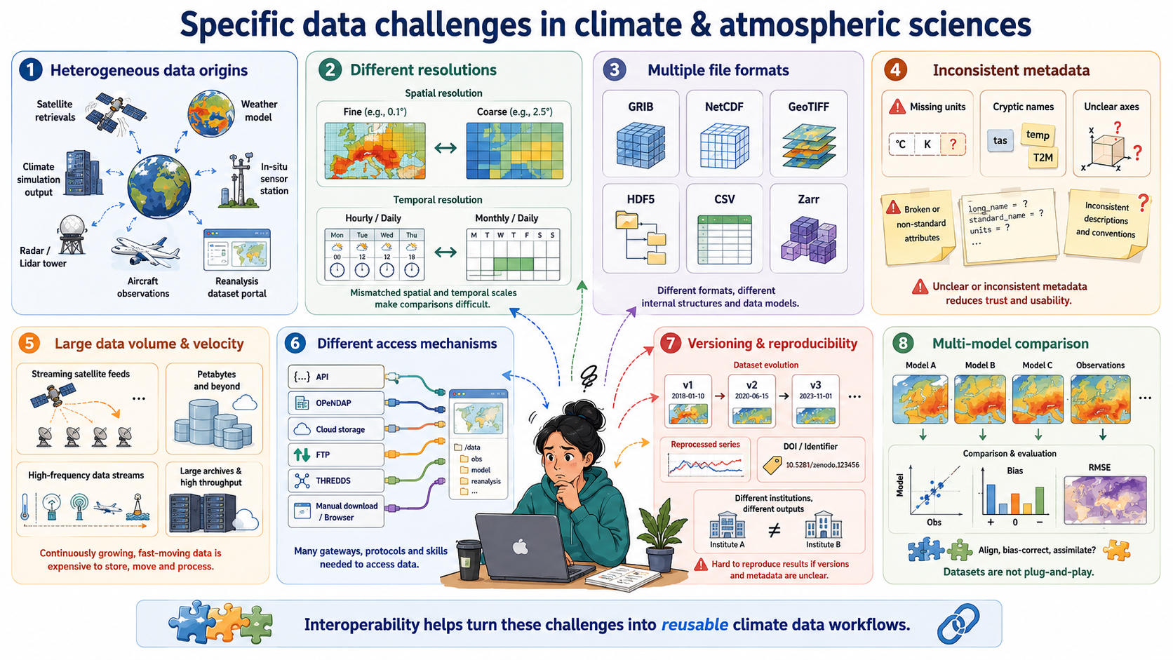
Specific data challenges in the climate & atmospheric sciences

Heterogeneous data origins: Climate research integrates satellite retrievals, weather models, climate simulations, in-situ sensors, radar, lidar, aircraft measurements, and reanalysis datasets—each with its own structure, conventions, and processing workflows.
Different spatial and temporal resolutions: Satellite images may be daily or hourly at 1 km resolution, while climate models may provide monthly or daily outputs on coarse grids; combining them requires consistent metadata and alignment.
Multiple file formats and data models: Data may come as GRIB, NetCDF, GeoTIFF, HDF5, CSV, or Zarr, each with different structural assumptions that affect processing and interpretation.
Inconsistent metadata quality: Missing units, inconsistent variable names, unclear coordinate systems, or non-standard attributes are frequent issues—making semantic interoperability a major challenge.
Large data volume and velocity: Earth observation missions (e.g., Sentinel, GOES), reanalysis products (ERA5), and high-resolution climate simulations produce terabytes to petabytes of data, making efficient, interoperable access necessary.
Different access mechanisms and services: Data are distributed across portals using APIs, OPeNDAP servers, cloud object storage, FTP, THREDDS catalogs, proprietary download tools, or manual interfaces, requiring technical interoperability to automate workflows.
Versioning and reproducibility issues: Climate datasets evolve frequently (e.g., reprocessed satellite series, new CMIP6 versions), and without stable identifiers or catalog metadata, reproducibility becomes difficult across institutions.
Need for multi-model and multi-dataset comparisons: Studies such as model evaluation, bias correction, and data assimilation depend on aligning diverse datasets that were never originally designed to work together.

Challenge

Discuss with you peer:

Participants inspect a small dataset and answer:

SH

• What is its structure?

• What metadata does it have?

• How is it accessed?

Show me the solution

Participants should identify whether the dataset is interoperable based on the three layers discussed (structural, semantic, technical).

dataset 1: Interoperable

Structure: NetCDF format with clear dimensions and variables.
Metadata: CF-compliant attributes, standard names, units.
Access: OPeNDAP protocol for remote access.

dataset 2: Not interoperable

Structure: CSV files with ambiguous column headers.
Metadata: Lacks standardized metadata, unclear variable meanings.
Access: Manual download, no API or remote access.

dataset 3: Not interoperable

Structure: NetCDF format but missing CF compliance.
Metadata: Inconsistent or missing units, unclear variable names.
Access: OPeNDAP protocol

Key Points

Interoperability ensures that data can be understood, combined, accessed, and reused across tools, institutions, and workflows with minimal manual intervention.
Interoperability operates at three complementary layers:structural (how data is encoded and organized),semantic (how data is described and interpreted), and technical (how data is accessed and exchanged).
The FAIR interoperability principles I1–I3 primarily address the semantic layer. They provide essential guidance on shared metadata languages, vocabularies, and references, but they do not fully cover structural and technical interoperability.
In climate and atmospheric science, all three layers are required for practical reuse. Structural standards (e.g., NetCDF, Zarr), semantic conventions (e.g., CF), and technical mechanisms (e.g., APIs, OPeNDAP, THREDDS) must work together.
Many real-world barriers to reuse datasets (unclear metadata, missing units, inconsistent coordinate systems, incompatible file formats, unstable access mechanisms) are failures of one or more interoperability layers.
Interoperable research workflows rely on established community formats, standardized metadata conventions, stable access protocols, and scalable cloud-native layouts that allow large heterogeneous datasets to be aligned, streamed, and analysed consistently.
Interoperability is essential in climate science because datasets come from diverse sources (models, satellites, sensors, reanalysis) and must be combined into integrated analyses that are reproducible and machine-actionable.

Wilkinson, M. D., Dumontier, M., Aalbersberg, I. J., Appleton, G., Axton, M., Baak, A., … & Mons, B. (2016). The FAIR Guiding Principles for scientific data management and stewardship. Scientific data, 3(1), 1-9.↩︎

Content from Structural interoperability

Last updated on 2026-10-08 | Edit this page

Estimated time: 60 minutes

Overview

Questions

What is structural interoperability, and what does it allow software to do?
How do data models, file formats, schemas, conventions, and access methods differ?
How can simple tabular formats such as CSV and TSV support reusable, machine-actionable data?
Which structural standards are appropriate for common climate and atmospheric data types?
What structural contract does the NetCDF data model provide?

Objectives

By the end of this episode, learners will be able to:

Explain structural interoperability as a shared, machine-actionable agreement about how data elements are organised and related.
Distinguish between a data model, encoding or file format, schema, community convention, and access method.
Evaluate the structural strengths and limitations of CSV/TSV, Parquet, NetCDF, Zarr, GRIB, and GeoTIFF.
Identify the additional information needed to make tabular data reliably reusable across tools.
Analyse a NetCDF dataset by identifying its dimensions, coordinate variables, data variables, attributes, and data types.

What is structural interoperability?

Structural interoperability concerns the organisation and representation of data: what kinds of data objects exist, how they are encoded, and how their relationships are expressed. A dataset is structurally interoperable when different software tools can reliably determine how the data are organised and process that organisation without needing undocumented instructions from the person who created it. For example, software may need to determine:

what records, columns, arrays, variables, or coordinates are present;
their data types, shapes, and dimensions;
how different data objects relate to one another;
which values represent missing data; and
whether the dataset follows expected structural rules.

A useful guiding question is:

Can another tool determine how the dataset is organised and process that organisation without bespoke instructions from the person who created it?

Structural interoperability does not mean that software automatically understands the scientific meaning of every value. For example, a program may recognise that air_temperature is a floating-point variable organised across time, latitude, and longitude. Understanding that the variable represents air temperature, which units apply, or whether it is scientifically comparable with another temperature variable involves semantic interoperability. Similarly, being able to retrieve the dataset from a remote server concerns technical interoperability. Structural interoperability sits between these layers: it makes the organisation of the data predictable and machine-actionable.

Structural interoperability is a shared data contract

A file extension such as .csv, .nc, .tif, or .zarr tells software something about how data may be represented, but the extension alone does not make a dataset structurally interoperable. Structural interoperability depends on a shared contract about how data are organised. At the centre of this contract is the data model: the logical structure that software expects to find.

Choosing a structural representation

Different formats provide different structural contracts.

Format or standard	Primary data model	Structural strengths	Additional requirement or limitation
CSV / TSV	Rows, columns, cells	Simple, human-readable, broadly supported	Types, missing values, units, dialect, and relationships usually require additional rules or a schema
Parquet	Typed, column-oriented tables	Stores a schema and physical types; supports efficient column selection and compression	Scientific meaning, units, coordinate systems, and domain constraints require additional metadata
NetCDF	Named multidimensional variables, dimensions, and attributes	Self-describing array structure; variables can share dimensions	Scientific coordinates and variable meaning usually require conventions such as CF
Zarr	Chunked, typed N-dimensional arrays and groups	Explicit shape, type, chunk organisation, fill values, and codecs	Scientific coordinate relationships and dimension conventions require additional agreements
GRIB2	Message-oriented meteorological fields	Strict templates and WMO code tables support operational exchange	Highly specialised for meteorological and forecast data
GeoTIFF	Georeferenced raster	Combines raster organisation with georeferencing	Scientific metadata beyond raster and georeferencing may require additional conventions
COG	GeoTIFF with an access-oriented physical layout	Enables efficient partial retrieval over HTTP	It is a GeoTIFF profile rather than a general scientific metadata model
GeoPackage	Geospatial tables, features, rasters, and tiles	Defines tables, constraints, coordinate reference systems, and extension mechanisms	Not designed primarily for large multidimensional climate arrays

There is therefore no universally “best” structural format.

The choice of data model reflects how you conceptualise the scientific data. Then choose a representation that preserves that structure with the least amount of flattening, reconstruction, or artificial complexity.

If I think of my data as…	Natural model
“a collection of observations”	Tabular
“variables varying along several shared dimensions”	Multidimensional arrays
“a collection of meteorological forecast fields”	GRIB
“a georeferenced spatial surface”	Raster
“geographic objects with properties”	Geospatial features

Callout

CSV and TSV: portable, but weakly self-describing

CSV and TSV are widely used because they are simple text formats that can be opened by spreadsheets, databases, statistical software, command-line tools, and most programming languages.

RFC 4180 documents a commonly used CSV syntax and the text/csv media type.

Consider this small dataset:

station_id,timestamp,air_temperature
NL001,2026-07-13T12:00:00Z,18.4
NL001,2026-07-13T13:00:00Z,18.8

Most software can immediately recognise rows and columns.

However, the file itself may not unambiguously tell a reader:

which data types the columns contain;
which unit is used for air_temperature;
what represents a missing value;
whether station_id has uniqueness constraints;
whether the timestamps are required to use a particular date-time format; or
whether identifiers refer to records in another table.

Even some properties needed to parse tabular text reliably can vary between files, including delimiters, quote characters, character encodings, decimal marks, and the presence of a header row.

CSV therefore provides excellent syntactic portability, but only a limited structural contract by itself.

That contract becomes stronger when the producer provides explicit rules such as:

stable column names;
explicit data types and constraints;
an unambiguous missing-value policy;
standard date and time representations;
stable identifiers and relationships; and
a machine-readable schema.

Two examples are W3C CSV on the Web and Frictionless Table Schema.

TSV follows the same tabular model but uses tabs rather than commas as delimiters.

The important point is therefore not that CSV is “non-interoperable.”

CSV is highly exchangeable, but weakly typed and weakly self-describing.

A carefully structured CSV accompanied by a machine-readable schema can be more interoperable than a poorly organised dataset stored in a more sophisticated binary format.

Challenge

Which structural contract is missing? — Think, Pair, Discuss

For each case, identify:

what a general-purpose software tool can already determine; and
what additional structural information would improve interoperability.

Case 1

rainfall.csv contains:

station,date,value

Case 2

radar.h5 contains several groups and arrays but follows no published schema or community convention.

Case 3

temperature.nc contains dimensions, variables, and attributes but does not declare a metadata convention.

Case 4

satellite.tif contains image pixels but no coordinate reference system or geotransform.

Case 5

forecast.zarr contains chunked arrays with known shapes and data types, but the relationships among those arrays are not documented.

Show me the solution

1. rainfall.csv

Software can recognise rows and columns.

Additional information could specify data types, date representation, units, missing values, identifier constraints, and relationships with other tables. A CSVW or Frictionless schema could provide much of this information.

2. radar.h5

An HDF5 reader can inspect groups, datasets, shapes, data types, and stored attributes.

However, HDF5 permits many possible organisational structures. Without a shared schema or convention, software cannot assume what the groups and arrays represent or how they relate.

3. temperature.nc

A NetCDF reader can determine variables, dimensions, shapes, types, and attributes.

Additional conventions may still be necessary to identify coordinates, standard scientific quantities, units, grid mappings, and other domain-specific relationships consistently. In climate science, CF Conventions commonly provide these rules.

4. satellite.tif

An image reader can decode the pixel grid.

Without georeferencing information, however, geospatial software cannot determine where that grid belongs on Earth. GeoTIFF provides standard mechanisms for encoding coordinate reference and spatial transformation information.

5. forecast.zarr

A Zarr implementation can find arrays, decode chunks, and determine shapes and data types.

Additional conventions are still needed to identify shared dimensions, coordinate arrays, scientific variables, units, and grid mappings consistently.

NetCDF: a shared data model for multidimensional scientific data

NetCDF — Network Common Data Form — is designed for storing and exchanging array-oriented scientific data. Its importance for structural interoperability comes from its shared data model. Rather than allowing every dataset creator to invent an arbitrary internal organisation, NetCDF defines a set of structural objects that software can inspect consistently. This allows different software tools to recognise how multidimensional data are organised without requiring dataset-specific instructions.

NetCDF was born from an interoperability problem

NetCDF originated at Unidata, part of the University Corporation for Atmospheric Research (UCAR) in the United States, at the end of the 1980s. The motivation was practical: Unidata needed a common way for different applications and computer systems to access and exchange real-time meteorological data. In 1987, Unidata organised a workshop to explore ideas from NASA’s Common Data Format (CDF). Building on these ideas, Glenn Davis and Russ Rew developed the first versions of NetCDF, with the format coming into use around 1989. The original goal was therefore not simply to invent another file format. NetCDF was designed to provide a portable, self-describing interface for array-oriented scientific data, allowing the same data to be accessed by different software, programming languages, and computer systems.

NetCDF was born from an interoperability question: how can scientists store multidimensional data once and allow different tools and computers to understand its structure?

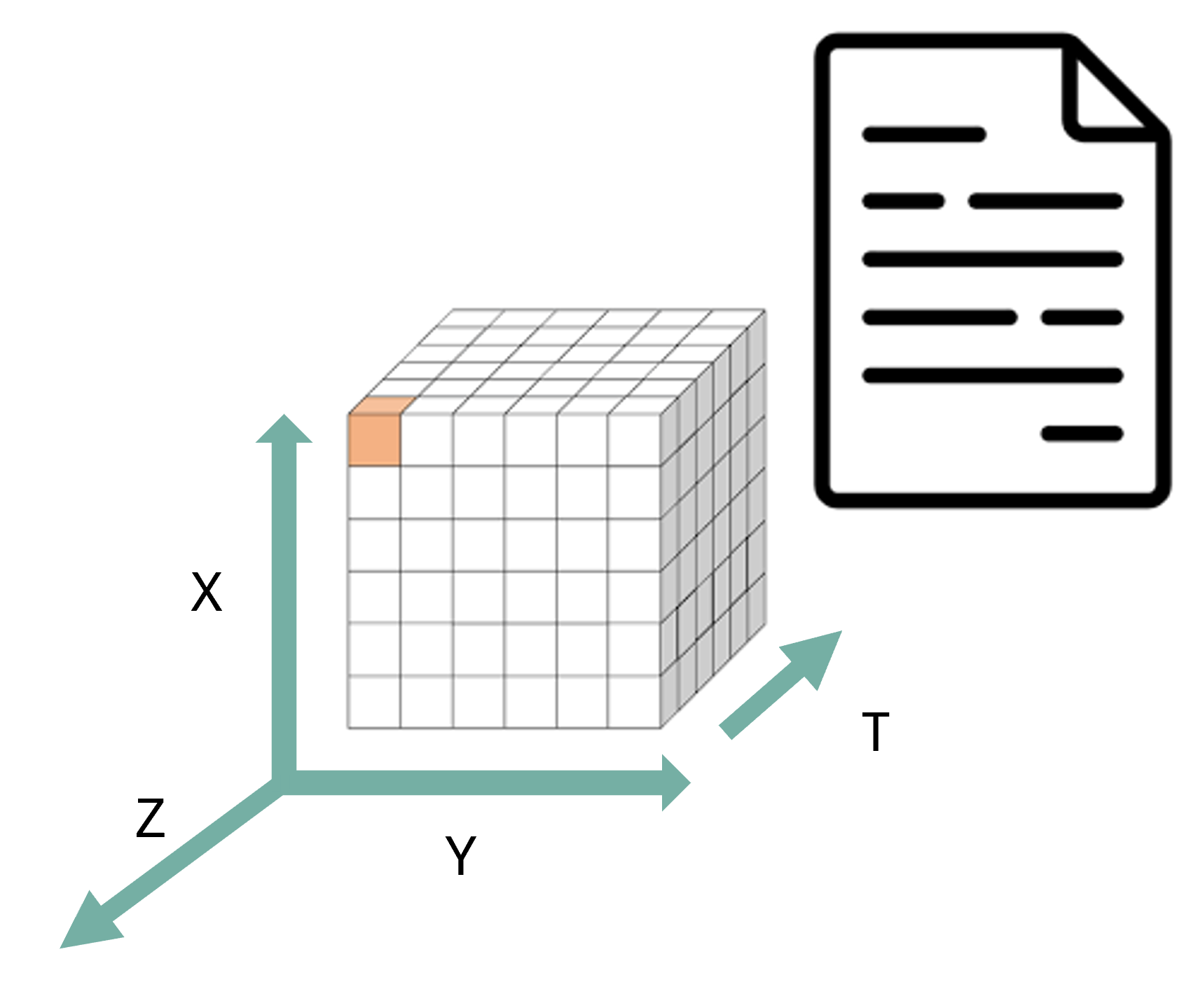
The classic NetCDF data model answers this question using three central structural elements: dimensions, variables, and attributes.

Dimensions

Dimensions define named axes and their lengths.

For example:

time = 24
latitude = 180
longitude = 360

Dimensions describe the shape of the dataset and allow different variables to refer to the same axes.

For example, both temperature and pressure measurements may vary over the same time, latitude, and longitude dimensions.

Variables

Variables are typed N-dimensional arrays whose shapes are defined using dimensions.

For example:

float air_temperature(time, latitude, longitude)

This declaration tells software that air_temperature:

contains floating-point values;
has three dimensions; and
is organised along the shared axes time, latitude, and longitude.

Another variable can reuse the same dimensions:

float surface_pressure(time, latitude, longitude)

The two variables are therefore structurally related through their shared dimensions. Software does not need to infer this relationship from where the values happen to occur in the file: the relationship is explicitly represented by the NetCDF data model.

Attributes

Attributes store metadata associated either with individual variables or with the dataset as a whole.

For example, variable-level attributes might include:

air_temperature:units = "K"
air_temperature:_FillValue = -999.0

A global attribute can describe the dataset itself:

title = "Atmospheric observations"

Attributes therefore provide additional information about variables or about the dataset without changing the dimensional structure of the arrays. The enhanced NetCDF-4 data model additionally supports groups, additional data types, multiple unlimited dimensions, and user-defined types.

A NetCDF file consists of dimensions, variables, and attributes

What software can determine from NetCDF

Because dimensions, variables, and attributes follow the NetCDF data model, a NetCDF reader can programmatically inspect:

dimension names and lengths;
variable names, data types, and shapes;
which dimensions are shared between variables;
variable-level and global attributes;
fill values and storage encodings; and
in NetCDF-4, groups and chunking information.

Consider again:

float air_temperature(time, latitude, longitude)

A NetCDF-aware tool can determine that air_temperature is a three-dimensional floating-point array and that its values are organised according to the dimensions time, latitude, and longitude. This is what makes NetCDF self-describing at the structural level.

The structure required to read the dataset is stored with the data rather than depending entirely on an external README or instructions from the researcher who created it.

What NetCDF does not guarantee

Being a valid NetCDF dataset does not guarantee that every climate-science application will interpret its scientific content consistently. NetCDF defines how dimensions, variables, data types, and attributes can be represented, but it does not by itself require communities to use the same:

coordinate rules;
variable names;
scientific units;
grid descriptions;
missing-value practices; or
terminology for physical quantities.

For example, all of the following could be syntactically valid NetCDF variable names:

temp
temperature
air_temp
T

NetCDF can tell software that these are variables and describe their data types, dimensions, and attributes. However, the NetCDF data model alone does not guarantee that software will understand that they represent the same physical quantity.

For climate and atmospheric data, the Climate and Forecast Metadata Conventions provide additional community rules for describing coordinates, scientific variables, units, grid mappings, cell bounds, and other metadata.

This gives us an important distinction: NetCDF provides a shared multidimensional data model; CF provides a more specific community contract for using that model consistently.

Inspecting the structure of a real NetCDF dataset

We can now apply these concepts to an atmospheric radar dataset.

The IDRA dataset is exposed through OPeNDAP, which allows us to inspect its NetCDF structure remotely.

Challenge

Identify the structural elements in a NetCDF dataset

Open the OPeNDAP inspection page for the IDRA dataset:

IDRA raw data, 2 January 2019

Identify:

the global attributes;
the dimensions and their lengths;
the coordinate variables;
three data variables and their dimensions;
the data types of those variables;
one variable-level attribute that controls the representation of missing data; and
any variables that appear to contain descriptive metadata as data values rather than as global attributes.

Show me the solution

1. Global attributes

The dataset-level attributes include:

title
institution
history
references
Conventions
location
source
example

The Conventions attribute declares:

CF-1.4

This declaration indicates that the producer intends the dataset to follow CF version 1.4.

The declaration itself does not demonstrate conformance; that requires checking the file against the convention.

2. Dimensions

The OPeNDAP Data Descriptor Structure shows:

time_raw_data = 73728
sample_beat_signal = 1024
time_processed_data = 144
range = 512
scalar = 1

3. Coordinate variables

Variables whose names match their corresponding dimensions include:

time_raw_data(time_raw_data)
sample_beat_signal(sample_beat_signal)
time_processed_data(time_processed_data)
range(range)

The scalar dimension does not have a variable named scalar. It is used as a length-one dimension by several variables.

4. Example data variables and dimensions

Examples include:

i_hh(time_raw_data, sample_beat_signal)

noise_power_horizontal(range)

equivalent_reflectivity_factor(time_processed_data, range)

radial_velocity(time_processed_data, range)

azimuth_processed_data(time_processed_data)

The variable declarations therefore expose how each variable relates to the dataset’s dimensions.

5. Example data types

Examples include:

i_hh                          16-bit integer

time_processed_data           64-bit real number

equivalent_reflectivity_factor
                              32-bit real number

range                         32-bit integer

6. Missing-data representation

Several processed radar variables, including equivalent_reflectivity_factor, differential_reflectivity, radial_velocity, and spectrum_width, declare:

_FillValue: -999.0

The existence, location, and type of _FillValue are part of the dataset’s structural representation.

What should happen analytically to a missing observation — for example whether it should be excluded or interpolated — is a separate analytical decision.

7. Metadata stored as variables

The dataset also contains string variables such as:

iso_dataset
product
station_details

These are variables containing descriptive text.

They should therefore not be confused with the global attributes listed at the dataset level.

The file is structurally inspectable because software can discover named dimensions, typed variables, shared axes, and attached attributes without bespoke instructions.

Whether every scientific variable and coordinate is described consistently according to CF is a different question. That takes us from structural interoperability towards semantic interoperability.

Callout

Can Ash compare two radar datasets from different years?

Ash wants to compare two IDRA radar datasets:

Both datasets are stored as NetCDF and exposed through OPeNDAP.

That already tells Ash two useful things:

the same family of software can inspect their NetCDF structures; and
the same access protocol can retrieve them.

But it does not prove that the datasets can simply be combined.

Ash still needs to compare properties such as:

variable names and data types
dimensions and dimension order
coordinate variables and coordinate values
fill values and missing-data representations
units and scaling attributes
declared conventions
variables present or absent in each dataset

This highlights three different interoperability questions:

Question	Interoperability layer
Can the same software and protocol retrieve the datasets?	Technical interoperability
Are the arrays, dimensions, coordinates, types, and metadata organised according to compatible rules?	Structural interoperability
Do the variables represent scientifically comparable quantities using compatible definitions and units?	Semantic interoperability

Structural interoperability reduces the amount of dataset-specific code required to compare the files. It does not remove the need to determine whether their scientific contents are genuinely comparable.

Key Points

Structural interoperability is a shared, machine-actionable contract about how data objects are organised, typed, related, and represented.
A file extension alone does not provide that contract: data models, encodings, schemas, and community conventions play different roles.
The appropriate representation depends on the underlying data model; tables, multidimensional arrays, meteorological fields, and rasters have different structural requirements.
CSV and TSV are highly portable but weakly self-describing; schemas and explicit structural rules make them more predictable for software.
NetCDF provides a shared multidimensional array data model based on dimensions, variables, and attributes.
NetCDF makes dataset structure machine-actionable, while conventions such as CF add community rules needed for consistent scientific interpretation.
Structural interoperability does not by itself guarantee semantic compatibility or technical accessibility.

Content from Semantic interoperability

Last updated on 2026-09-02 | Edit this page

Estimated time: 45 minutes

Overview

Questions

What is semantic interoperability?
What types of meaning must be made explicit to enable semantic interoperability?
Why can two structurally similar datasets still be scientifically incompatible?
What is the difference between a label, a controlled vocabulary, a code list, and an ontology?
Where can researchers discover, evaluate, and share semantic artefacts for the Earth sciences?
How do the CF Conventions encode the meaning and context of climate and atmospheric data?
Is using the same CF standard_name sufficient to make two variables directly comparable?
What does it mean for a NetCDF file to conform to a particular version of the CF Conventions?
What can a CF compliance checker determine, and what are its limitations?

Objectives

By the end of this episode, learners will be able to:

distinguish structural interoperability from semantic interoperability;
identify the semantic information needed to interpret and compare scientific variables;
distinguish free-text labels from controlled vocabulary terms and formally defined relationships;
use an Earth-science semantic-artefact catalogue to discover and critically assess relevant ontologies and vocabularies;
explain how CF standard names, units, coordinates, bounds, grid mappings, and cell methods work together;
evaluate whether two variables with similar names are semantically and scientifically comparable;
interpret CF compliance-checker findings critically, including version mismatches and tool limitations; and
identify semantic gaps in the IDRA radar datasets that may need harmonisation before comparison.

What is semantic interoperability?

Semantic interoperability concerns shared and explicit meaning.

A dataset is semantically interoperable when different people and software systems can interpret its variables, categories, relationships, and measurement context consistently because those meanings are expressed using documented, community-agreed terms and rules.

A useful guiding question is:

Can another researcher or software tool determine what the values represent, under which conditions they were produced, and how they relate to other data without relying mainly on tacit knowledge?

Or in other words : Can others understand and reuse the data correctly without making unnecessary assumptions?

This definition does not require every explanation to be written directly inside one file. Meaning may also be expressed through persistent identifiers that resolve to external vocabularies, code lists, specifications, instruments, methods, or provenance records. What matters is that the references and relationships are explicit and machine-actionable rather than hidden in personal knowledge, filenames, or informal documentation.

Semantic interoperability supports questions such as:

What physical quantity is represented?
What entity, medium, or phenomenon does the quantity concern?
What is the direction or reference frame?
At which height, depth, pressure level, or location was it observed?
Does each value represent a point measurement, mean, sum, minimum, maximum, or another statistic?
Over which spatial or temporal interval was it calculated?
Which calendar, coordinate reference system, or vertical datum is used?
Which quality flag, uncertainty estimate, instrument, or processing step applies?
Are two variables equivalent, convertible, related, or fundamentally different?

Structure and meaning are different—but connected

Structural interoperability and semantic interoperability address different questions.

Question	Primarily structural	Primarily semantic
Does a variable exist, and what is its data type?	✓
Which dimensions does the variable use?	✓
Where is the `units` attribute stored?	✓
What physical quantity does the variable represent?		✓
Is `K` dimensionally compatible with `degC`?		✓
Does `time: mean` describe an average rather than an instantaneous value?		✓
Which coordinate variable applies to a data variable?	✓	✓
Does a height coordinate refer to metres above ground, sea level, or another reference surface?		✓
Is a quality-control variable explicitly related to the measurement variable?	✓	✓

The boundary is not always absolute. A metadata convention often defines both:

structural rules, such as where an attribute must occur or how a related variable is referenced; and
semantic rules, such as what the permitted term means.

For example, the presence and location of a cell_methods attribute are structural. The distinction between time: point, time: mean, and time: sum is semantic.

Semantic resources for expressing shared meaning

Scientific meaning can be expressed using different types of semantic resources. These resources vary in how formally they define terms and relationships.

Common examples include:

Free-text labels — human-readable descriptions, such as long_name = "surface temperature". They provide useful context but are not necessarily standardised.
Controlled vocabularies — agreed sets of terms with documented definitions, such as the CF Standard Name Table.
Code lists — predefined values or codes used for a particular property or category.
Taxonomies and thesauri — collections of concepts organised through relationships such as broader, narrower, or related terms.
Ontologies — formal representations of concepts and the relationships between them, enabling richer machine-readable descriptions.
Persistent identifiers and qualified references — links that connect a dataset or metadata element to an authoritative definition, instrument, method, vocabulary term, or other related resource.

These resources are not interchangeable. The appropriate choice depends on what meaning needs to be expressed and how precisely software needs to interpret it.

The CF Standard Name Table is a controlled vocabulary. It defines standard names, descriptions, and canonical units. It is not, by itself, a full ontology of climate science.

A semantic resource is more useful when:

its terms have stable identifiers;
definitions are publicly accessible;
versions and changes are documented;
synonyms and deprecated terms are managed;
relationships between concepts are explicit where needed; and
the resource is maintained through an open community process.

This aligns with the FAIR Interoperability principles: data and metadata should use formal, shared knowledge-representation languages, FAIR vocabularies, and qualified references to related data and metadata.

Callout

Relevant resource: EarthPortal

EarthPortal is a catalogue and repository for ontologies and other semantic artefacts in Earth-system, environmental, and related domains. It can help researchers, data stewards, and infrastructure developers move beyond locally invented labels by discovering semantic resources that may already exist in their community.

EarthPortal provides several ways to explore and evaluate semantic artefacts:

Browse the ontology catalogue and filter resources by Earth-science category, group, language, representation format, or semantic-resource type.
Search ontology content to find concepts across multiple ontologies rather than searching only by ontology title.
Use the Recommender to identify potentially relevant ontologies from a sample of terms or text.
Use the Annotator to identify ontology concepts that may describe terms occurring in documentation or metadata.
Inspect mappings, identifiers, classes, properties, provenance, submissions, and available machine-readable representations.
After creating an account and signing in, use Submit ontology to share an ontology or another semantic artefact with the wider Earth-science community.

A useful search exercise is to look for terms such as air_temperature, precipitation_flux, or radar-related quantities and compare what EarthPortal exposes with the current CF Standard Name Table.

Semantic interoperability is not provided by a file format

NetCDF, Zarr, CSV, TSV, Parquet, GeoTIFF, and other formats can all carry data that are semantically clear - or semantically ambiguous.

For example, a CSV table may contain:

station,time,RR
Cabauw,2026-07-14T08:00:00Z,0.3

The table is structurally simple, but RR remains ambiguous unless a schema or metadata record states:

the controlled concept represented by RR;
whether the value is precipitation amount, rainfall depth, or precipitation rate;
the unit;
the time interval;
whether the value is instantaneous, accumulated, averaged, or derived;
the station identifier and coordinate reference; and
how missing and quality-controlled values are represented.

A Parquet schema can define RR as a floating-point column, but a data type does not define the scientific quantity. A NetCDF variable can carry attributes, but the presence of attributes does not ensure that they use shared terms correctly.

The file format provides a place to encode meaning. A community convention supplies the semantic contract.

Semantic interoperability requires context, not only names and units

Consider two variables:

float temperature(time, latitude, longitude);
    temperature:standard_name = "air_temperature";
    temperature:units = "K";

and:

float tas(time, latitude, longitude);
    tas:standard_name = "air_temperature";
    tas:units = "degC";

The variable names differ, but the shared standard_name indicates the same physical quantity. Their units are convertible, so software can harmonise them.

However, this does not yet prove that the variables can be directly combined. Ash must still inspect:

the height or pressure level of the air temperature;
coordinate systems and locations;
time coordinates and calendars;
spatial and temporal resolution;
whether values are instantaneous or averaged;
cell bounds and aggregation intervals;
observation versus model context;
quality flags and uncertainty;
calibration and processing level; and
missing-data and validity rules.

Semantic interoperability establishes interpretable meaning and relationships. It does not automatically establish that two datasets are scientifically interchangeable or suitable for a particular analysis.

Challenge

Can these variables be compared? (Think–Pair–Discuss)

Consider the following variables.

Dataset A

standard_name = "air_temperature"
units = "K"
height = 2 m
cell_methods = "time: point"

Dataset B

standard_name = "air_temperature"
units = "degC"
height = 2 m
cell_methods = "time: mean"
time_bounds = one-hour intervals

Dataset C

standard_name = "surface_temperature"
units = "K"
cell_methods = "time: point"

Discuss:

Which pairs describe the same physical quantity?
Which units are convertible?
Which variables can be directly compared without further processing?
What harmonisation would be required?
Which information is semantic, and which is structural?

Show me the solution

Datasets A and B

They use the same standard name and refer to air temperature at the same height. Their units are convertible. However, Dataset A represents point values while Dataset B represents one-hour means. They should not be treated as directly equivalent until their temporal representation is harmonised—for example, by calculating comparable hourly means from Dataset A, if its sampling supports that operation.

Datasets A and C

Their units are compatible, but the standard names identify different quantities. air_temperature and surface_temperature must not be treated as synonyms.

Datasets B and C

The variables differ in physical quantity and temporal treatment, so unit conversion alone is insufficient.

Structural information

The existence and location of attributes, the link to time_bounds, and the shapes and dimensions of variables are structural.

Semantic information

The definitions of air_temperature, surface_temperature, time: point, time: mean, the height reference, and the interpretation of units are semantic.

Semantic interoperability through the CF Conventions

The Climate and Forecast (CF) Metadata Conventions provide standard ways to describe the meaning and context of variables in NetCDF datasets. This helps researchers and software determine what the data represents and where and when it applies.

Some of the main CF elements are:

standard_name — What is being measured? Gives a variable a standardised name with a defined scientific meaning, such as air_temperature or precipitation_flux.
long_name — How can we describe it for people? Provides a human-readable description of the variable.
units — How are the values expressed? Specifies the physical units of the variable. When a standard_name is used, the units must be physically compatible with its canonical units.
Coordinates — Where and when? Describe the spatial and temporal location of the data, including latitude, longitude, vertical position, and time.
bounds and cell_methods — What does each value represent? bounds can describe the extent of a coordinate interval, while cell_methods describes operations such as a mean, sum, or maximum over space or time.
grid_mapping — How is the data located on Earth? Describes the coordinate reference system or map projection used by the dataset.
Ancillary variables and flags — What additional information is associated with the values? Can describe information such as measurement uncertainty, instrument status, or quality-control flags.
featureType — What kind of observations are these? Describes discrete sampling geometries such as time series, profiles, or trajectories.

Together, these elements make the scientific meaning and context of the data more explicit and machine-readable.

Callout

Explore further: the Climate and Forecast ontology representation

EarthPortal includes the Climate and Forecast (CF) features ontology, an OWL representation of generic features derived from the CF Standard Names vocabulary. It exposes CF-related concepts through ontology classes, properties, individuals, identifiers, and relationships that can be explored programmatically or through the portal interface.

This resource illustrates the difference between:

the authoritative CF Standard Name Table, which governs the standard names used in CF-compliant datasets; and
an ontology representation, which expresses selected CF concepts and relationships in a formal knowledge-representation language.

The ontology representation may support linked-data exploration, mappings, semantic annotation, and integration with other ontologies. However, it should not automatically be treated as a replacement for the current CF Standard Name Table or the CF Conventions.

CF is a convention, not a complete description of every research context

CF is powerful, but CF compliance does not guarantee:

that the scientific values are correct;
that calibration or processing was appropriate;
that uncertainty is adequately described;
that all provenance is available;
that discovery metadata are complete;
that two datasets use the same spatial or temporal resolution;
that two variables are suitable for the same research question;
that missing values are acceptably limited; or
that a dataset is free from software or production errors.

Other standards and metadata profiles may complement CF by providing richer dataset level discovery and citation metadata. For example:

dataset-discovery metadata may be expressed through Attribute Convention for Data Discovery (ACDD, see Glossary), ISO 19115 (Geographic information metadata , see Glossary), DataCite (see Glossary), or repository metadata;
instruments and observation procedures may require domain-specific vocabularies or provenance models;
persistent identifiers can connect datasets to instruments, software, methods, publications, and derived products.

Semantic interoperability is therefore layered. CF provides an important domain convention, not the totality of scientific meaning.

Challenge

Semantic interoperability: True or False?

Indicate whether each statement is True or False, and justify your answer.

A NetCDF file with dimensions, variables, and units is semantically interoperable by default.
CF standard names allow software to distinguish different kinds of temperature.
Semantic interoperability mainly benefits human readers, not automated workflows.
Two datasets using the same CF standard name can always be compared directly without further interpretation.
Semantic interoperability can be achieved reliably through locally invented variable names, without community-agreed definitions.
A descriptive long_name has the same machine-actionable status as a valid CF standard_name.
Passing a compliance checker proves that a dataset is scientifically correct and fully interoperable.
Variables expressed in K and degC may be convertible while still requiring additional contextual harmonisation.

Show me the solution

False. NetCDF provides a self-describing structure, but dimensions and units do not fully define scientific meaning, context, statistical treatment, or relationships.
True. CF standard names distinguish concepts such as air_temperature, sea_surface_temperature, and surface_temperature through controlled terms and definitions.
False. Shared semantics enable automated discovery, validation, unit conversion, subsetting, comparison, and integration.
False. A shared standard name is strong evidence that variables represent the same physical quantity, but direct comparison still depends on coordinates, units, heights or depths, cell methods, bounds, resolution, quality, provenance, and processing context.
False. Local names may be understandable within one project, but reliable interoperability requires mappings to shared definitions, vocabularies, or identifiers.
False. long_name is normally free text. A CF standard_name must be selected from the governed Standard Name Table and has a defined meaning and canonical unit.
False. A checker evaluates implemented conformance rules. It does not verify scientific correctness, data quality, completeness of all relevant metadata, or suitability for a specific analysis.
True. Unit conversion may be possible, but the variables may still differ in height, aggregation, calendar, coordinate system, processing level, or measurement method.

What does CF-compliant mean?

A NetCDF file is CF-compliant relative to a declared CF version when it satisfies the requirements of that version and uses CF terms according to their defined meanings.

For example:

:Conventions = "CF-1.13";

The global Conventions attribute is a declaration by the data producer. It is not proof by itself. A file may declare a convention while still containing invalid standard names, incompatible units, missing coordinate metadata, or incorrectly expressed relationships.

CF documents distinguish between:

requirements, which must be satisfied for conformance; and
recommendations, which improve interoperability but are not always mandatory.

A compliance assessment should therefore report:

the CF version claimed by the file;
the CF version against which it was evaluated;
requirements that fail;
recommendations that are not followed;
warnings or implementation limitations; and
which checker and checker version produced the report.

Callout

Compliance is version-specific

A file written for an older CF version should ideally be evaluated against that version. Running a newer checker may still reveal useful interoperability problems, but it does not retroactively determine whether the file conformed to every rule of its originally declared version.

Similarly, a checker may implement only part of a convention. The CF specification remains the authoritative source.

Inspecting semantic metadata in the IDRA radar files

The two IDRA files used in this lesson declare:

Conventions = "CF-1.4"

They contain useful structural and descriptive metadata, including time coordinates, units, long_name values, comments, and fill values. However, several radar data variables—such as:

equivalent_reflectivity_factor
differential_reflectivity
radial_velocity
spectrum_width
differential_phase

are primarily described through local variable names, free-text long_name values, units, and comments.

This creates useful questions for semantic assessment:

Does each local variable name correspond to a valid CF standard name?
If a matching standard name exists, is it recorded in the standard_name attribute?
Are units written in a valid and unambiguous UDUNITS form?
Does ms-1 express the intended velocity unit, or should it be written as m s-1 or m/s?
Are azimuth, elevation, range, and radar position represented through sufficient coordinate semantics?
Is the positive direction of radial velocity explicit?
Are measurement uncertainties or quality flags linked to the data variables?
Do the files provide enough metadata to distinguish point measurements, averages, and derived products?
Does declaring CF-1.4 accurately describe how all variables use the convention?

The purpose is not to conclude that the datasets are unusable. They are structurally similar and richly documented for human readers. The purpose is to identify which meanings are machine-actionable and which still depend on domain knowledge or free-text interpretation.

Challenge

Ash’s semantic-comparison checklist

Ash wants to compare equivalent_reflectivity_factor and radial_velocity between the 2009 and 2019 IDRA files. One from 27 April 2009 and one from 2 January 2019.

Before combining the values, decide whether she has enough information to answer the following questions.

Question	Metadata element to inspect	Why it matters
Do both variables represent the same physical quantity?	`standard_name`, `long_name`, definition or vocabulary mapping	Similar local names are not proof of semantic equivalence
Are units valid and compatible?	`units`, canonical units, UDUNITS parsing	Strings that look similar may be invalid or ambiguous
Is the sign convention the same?	standard-name definition, comments, reference direction	Opposite sign conventions can reverse interpretation
Do values represent the same temporal treatment?	`cell_methods`, time bounds, sampling information	Point values and means are not equivalent
Are measurements located in the same coordinate frame?	range, azimuth, elevation, station position, CRS or grid mapping	Radar bins need spatial interpretation
Are missing and invalid values handled consistently?	`_FillValue`, `missing_value`, `valid_range`, quality flags	Invalid values must not enter comparisons
Are processing and calibration comparable?	`history`, provenance, processing-level metadata, instrument information	Identical names do not guarantee identical processing
Is uncertainty represented?	`ancillary_variables`, uncertainty variables, quality flags	Differences may be smaller than measurement uncertainty

Show me the solution

The two files use nearly identical variable names, dimensions, units, and comments, which strongly supports comparison using a shared workflow. However, semantic comparability should not be inferred from names alone.

Ash can establish more reliable comparability by:

validating or mapping the local radar variable names to controlled terms;
confirming unit syntax and compatibility;
documenting sign conventions and measurement geometry;
checking whether temporal and spatial sampling are equivalent;
comparing calibration, processing, and noise information;
applying missing-value and quality-control rules consistently; and
recording any assumptions made during harmonisation.

Callout

The IOOS Compliance Checker

The IOOS Compliance Checker is a Python-based tool that evaluates local or remote NetCDF datasets against implemented metadata standards, including selected versions of CF. Its source code and documentation are available through the IOOS Compliance Checker project.

The checker is useful for identifying potential conformance problems, but its own documentation states that it should be used as guidance rather than treated as the authoritative determination of complete compliance.

Run the assessment

Open the IOOS Compliance Checker.
Inspect the file before running the checker, to see which version of CF is using.
Select an available CF test version. Prefer a relatively close compatibility assessment.
Upload the .nc dataset. You can also provide a direct remote OPeNDAP data URL, if using the CLI.
Submit the dataset and download or save the report.
Classify each finding into one of the following categories:
- invalid or missing controlled-vocabulary term;
- invalid or incompatible unit;
- coordinate or reference-system problem;
- missing relationship between variables;
- missing statistical or interval context;
- recommendation for human-readable or discovery metadata;
- checker limitation or version mismatch.

Interpretation questions

Which CF version does the dataset claim?
Which CF version did the checker actually evaluate?
Which findings are errors, and which are recommendations or warnings?

Key Points

Semantic interoperability concerns shared, explicit, and machine-actionable meaning.
File formats and readable labels provide containers for meaning but do not guarantee semantic agreement.
Catalogues such as EarthPortal support the discovery, assessment, mapping, and sharing of Earth-science semantic artefacts, but users must still evaluate authority, versioning, provenance, licensing, and community adoption.
Controlled vocabulary terms, units, coordinates, bounds, cell methods, grid mappings, flags, and qualified relationships work together to express scientific meaning.
A CF standard_name identifies a physical quantity; long_name remains free text for human readability.
The same standard name and convertible units are not sufficient to guarantee direct scientific comparability.
CF compliance is relative to a specific version and does not prove scientific correctness, data quality, or suitability for a particular analysis.
The global Conventions attribute is a conformance claim, not evidence that every requirement is satisfied.
Compliance checkers evaluate implemented rules and must be interpreted alongside the authoritative specification and domain knowledge.
The IDRA files are structurally similar and well documented for human readers, but some radar semantics may still require controlled mappings, clearer unit syntax, measurement-context metadata, and provenance.
Semantic interoperability is achieved through community-agreed definitions, stable identifiers, explicit relationships, and transparent harmonisation—not through variable names alone.

Content from Technical interoperability: Data access protocols

Last updated on 2026-09-23 | Edit this page

Estimated time: 45 minutes

Overview

Questions

What is technical interoperability?
What is the difference between storing data remotely and providing remote data access?
What is the DAP (Data Access Protocol)?
How does OPeNDAP enable remote access without full download?
What happens when we open a remote NetCDF file using xarray.open_dataset()?
Why are remote data-access protocols important for large-scale scientific workflows?

Objectives

By the end of this episode, learners will be able to:

Define technical interoperability in the context of scientific data infrastructures.
Explain how DAP enables interoperable machine-to-machine data access.
Access a remote NetCDF dataset via OPeNDAP using Python.
Perform server-side subsetting of variables and dimensions.
Distinguish between metadata access and actual data transfer.

What is technical interoperability?

So far, we have considered whether scientific data are structured in a predictable way and whether their scientific meaning can be understood consistently. Technical interoperability introduces another question: How can one computer system access data held by another system? A dataset may be perfectly structured and well described, but that does not automatically mean that another system can access it efficiently.

Technical interoperability concerns the mechanisms that allow independent systems to communicate and exchange data through agreed technical interfaces and protocols.

Imagine, for example, that a climate dataset is stored in a research data repository. A researcher may be interested only in one variable, covering a particular period and geographical region. One possible approach is to download the complete file and perform the selection locally. Another possibility is for the remote infrastructure to provide a mechanism through which the researcher can request only the required part of the dataset. This second possibility is particularly important for large scientific datasets and repetitive automated computational workflows because software can request only the variables, time periods, or spatial regions needed for each analysis, avoiding repeated transfer and storage of complete datasets. Technical interoperability therefore concerns not only whether data can be transferred, but also how systems agree to request, exchange, and access those data across a network.

Storage is not the same as access

It is useful to distinguish where data are stored from how data are accessed. A NetCDF file may physically reside on institutional storage, repository infrastructure, object storage, or another remote storage system. However, knowing where the bytes are stored does not automatically tell us how researchers or software applications can interact with them. Between the storage system and the researcher there is often a data-access service. This service receives requests from clients, interacts with the underlying dataset, and returns the requested information. For example, a NetCDF file may be stored by a repository while a data server such as THREDDS or Hyrax makes that dataset accessible over the network. Scientific applications such as Python libraries can then communicate with the data server instead of directly interacting with the storage infrastructure. This service layer is an important component of technical interoperability.

A dataset being stored remotely, including in cloud infrastructure, therefore does not automatically make it technically interoperable. The infrastructure must also provide an agreed mechanism through which independent clients can access the data.

A protocol defines how data are accessed

A protocol is an agreed set of rules describing how systems communicate with each other. HTTP, for example, defines rules for exchanging resources across the Web. Scientific data access often requires more than transferring an entire file. A scientific client may need to discover which variables a dataset contains, inspect its dimensions and metadata, or request only a particular variable, time interval, depth level, or geographical subset. A scientific data-access protocol defines how these kinds of requests and responses are expressed between a client and a remote data service. This is different from the internal structure of the file itself. NetCDF defines how arrays, dimensions, variables, and attributes are organised within a dataset.

A protocol such as DAP defines how a remote client can discover and retrieve those structures across a network. The two therefore address different aspects of interoperability. NetCDF helps software understand how the dataset is structured, while DAP provides a standardized mechanism for accessing that structured dataset remotely.

Different protocols, different ways of accessing remote data

Remote data can be made available through different technical mechanisms. The simplest form is ordinary HTTP or HTTPS file access. In this case, the client requests a file and the server transfers that file to the client. This model works very well for many datasets, particularly when files are relatively small or when the researcher needs the complete dataset. Scientific data infrastructures can also offer more specialized access mechanisms. DAP and OPeNDAP, for example, allow clients to interact with the internal structure of scientific datasets and request selected variables or subsets instead of necessarily retrieving the complete file. Geospatial communities use other standardized services as well. The Open Geospatial Consortium has developed standards such as the Web Coverage Service, which can provide access to spatial and temporal subsets of multidimensional geospatial data.

These mechanisms do not necessarily compete with one another. The same dataset may be exposed through several access methods. A researcher might download a complete NetCDF file through HTTPS, while another researcher accesses selected variables from the same dataset through OPeNDAP. Data servers such as THREDDS are designed to support this type of architecture, allowing one underlying dataset to be exposed through multiple access services. In this episode, we focus on DAP and OPeNDAP, because they were specifically developed to support remote access to structured scientific datasets.

DAP and OPeNDAP

From distributed oceanography to remote data access

The origins of OPeNDAP go back to the early 1990s, when oceanographers were facing a problem that is still familiar today: important scientific datasets were distributed across researchers, institutions, and federal data centres, and different systems used different ways of storing and accessing them. The challenge was therefore not simply how to create another scientific file format. Formats such as NetCDF already provided mechanisms for representing structured scientific data. The problem was how researchers could access those distributed datasets through a common mechanism, regardless of where the data were physically stored.

A key moment came in 1993, when a workshop at the University of Rhode Island, involving researchers from URI and MIT and supported by NASA, NOAA, and The Oceanography Society, explored the requirements for what became the Distributed Oceanographic Data System (DODS). One of the remarkably simple ideas that emerged from this work was: A URL equals a dataset. and, even more importantly: A URL with constraints equals a subset. In other words, a scientific dataset could be treated as a resource accessible over the network, while additional information in the request could specify which part of that dataset should be returned. This principle anticipated the type of remote subsetting that is still central to OPeNDAP today.

By 1995, the first Distributed Oceanographic Data System had been implemented. DODS combined the emerging World Wide Web with a common data model and data-access protocol so that scientific applications could retrieve distributed data through a standardized interface. The technology was already being presented to the broader Web community in 1995, including at the Fourth International World Wide Web Conference. Although the project started in oceanography, its underlying problem was not specific to ocean data. Climate science, atmospheric science, remote sensing, Earth observation, and many other disciplines faced the same challenge of accessing large and distributed scientific datasets.

The technology therefore evolved from the oceanography-specific DODS into the more discipline-neutral Data Access Protocol (DAP) and the OPeNDAP software ecosystem. OPeNDAP Inc. was formed as a nonprofit organisation in 2000 to maintain and develop this infrastructure. There is an important terminology distinction between DAP, OPeNDAP, and the software that actually serves datasets. DAP is the protocol itself. It specifies how clients and servers communicate when accessing structured scientific data. OPeNDAP is the project and technology ecosystem responsible for developing DAP and associated software. A separate piece of software acts as the data server. The server implements the protocol and exposes datasets to remote clients. One example is Hyrax, the data server developed by OPeNDAP. Hyrax can expose supported scientific datasets through DAP. Another widely used data server in the Earth sciences is the THREDDS Data Server, which can also expose NetCDF datasets through OPeNDAP services. For researchers accessing existing datasets, the distinction may initially be invisible. They simply receive an OPeNDAP endpoint and use it from their scientific software.

For data providers and infrastructure operators, however, the distinction is important. Someone must operate the server that interprets DAP requests and connects those requests to the underlying scientific datasets. The main purpose, however, remained essentially the same: Allow independent scientific clients to access distributed structured data through a common protocol.

How DAP works

The Data Access Protocol (DAP) defines a common way for clients to inspect the structure and metadata of a remote dataset and request selected data from it. A client can first discover which variables, dimensions, and metadata are available. It can then request only the data required for a particular analysis, such as one variable, a particular time interval, selected depth levels, or a geographical subset. The remote data service interprets the request, interacts with the underlying dataset, and returns the requested information.

This standardized interaction means that the client and server can be developed independently. A Python application, for example, does not need to understand how the provider’s storage infrastructure works internally. Likewise, the data provider does not need to develop a special access mechanism for every possible analysis application. Both sides only need to understand the same protocol.

This separation is one of the main contributions of DAP to technical interoperability.

From DAP2 to DAP4

The protocol has continued to evolve as scientific data and infrastructures have become more complex. DAP2 became widely adopted and in 2005 was approved as a standard for NASA (National Aeronautics and Space Administration) Earth Science Data Systems. It remains common across existing scientific data infrastructures. In 2006, OPeNDAP released the first version of Hyrax, its data server implementation, allowing providers to expose scientific datasets through DAP services.

Later, DAP4 was developed to provide a richer data model capable of representing a broader range of modern scientific data structures. DAP4 was released in 2014 following collaboration involving OPeNDAP, Unidata, NOAA (National Oceanic and Atmospheric Administration), and NSF (National Science Foundation)-supported work.

For this episode, however, the detailed technical differences between DAP2 and DAP4 are less important than the interoperability principle they share: DAP provides a standardized conversation between a scientific data client and a remote data service.

Publishing a file is not the same as providing remote data access

Imagine two repositories containing exactly the same NetCDF file. The first repository allows users to download the file through HTTPS. The second repository provides the same download option but also exposes the dataset through DAP2 and DAP4.

From a structural interoperability perspective, both repositories may contain exactly the same NetCDF dataset. The variables, dimensions, attributes, and file structure have not changed. From a technical interoperability perspective, however, the access possibilities are different.

In the second repository, compatible scientific clients can inspect and retrieve selected parts of the dataset remotely. The repository therefore provides an additional technical access layer on top of the stored file. This distinction is important when selecting infrastructure for large multidimensional datasets.

Researchers should therefore ask not only: Can this repository store my NetCDF files? but also: How will machines be able to access the data after I publish them?

The file format and the repository access infrastructure solve different problems, and both contribute to the eventual reusability of the dataset.

Callout

What if the repository does not provide OPeNDAP?

A research institution, project, or infrastructure provider can also operate its own OPeNDAP-compatible server. Hyrax is an open-source data server developed by OPeNDAP for this purpose. An organisation can configure Hyrax to expose scientific datasets stored on its own infrastructure and make them available to compatible remote clients through DAP. Instead of seeing OPeNDAP only from the user’s perspective, participants can understand what happens on the provider side. A NetCDF file may initially exist only on local or institutional storage. Once a service such as Hyrax is configured to expose that file, clients elsewhere on the network can interact with it through a standardized DAP endpoint.

Technical interoperability is created by connecting data to interoperable services and protocols. It is not an intrinsic property of the storage location alone. However, operating Hyrax is not equivalent to depositing data in a trusted research data repository.

A repository typically provides preservation, persistent identifiers, metadata management, citation support, access governance, and long-term stewardship. Hyrax primarily provides a technical data-access service.

In a mature research infrastructure, these components can complement one another. The repository manages and preserves the research object, while a service such as THREDDS or Hyrax provides specialized machine access to its scientific contents.

For the purposes of this course, configuring Hyrax can therefore be treated as an optional provider-side example rather than as something every researcher is expected to operate themselves.

4TU.ResearchData: A repository that exposes NetCDF data through DAP

4TU.ResearchData provides a useful example of this architecture. NetCDF datasets deposited in the repository can be connected to a THREDDS infrastructure that exposes different access mechanisms for the same underlying data. A researcher can retrieve the complete file through an HTTP-based service when that is the most appropriate workflow. The same dataset can also be exposed through OPeNDAP using DAP2 or through DAP4, allowing compatible clients to interact with the dataset remotely. The researcher can therefore choose an access mechanism according to the computational task rather than being restricted to one method.

Hands-on: Accessing remote NetCDF datasets stored in 4TU.ResearchData using the DAP protocol

We now move from concept to practice.

We will use:

xarray
A remote OPeNDAP endpoint
A NetCDF dataset hosted on a THREDDS server
Jupyter Lab

Step 1 – Open a remote dataset

Open Jupyter Lab and choose the appropriate environment of the lesson (see Setup)
Launch Jupyter Lab, open a terminal and type:

BASH


jupyter lab

Open a new notebook
Check installed libraries

PYTHON


import xarray as xr

Open a dataset

PYTHON


url = "https://opendap.4tu.nl/thredds/dodsC/IDRA/2019/01/02/IDRA_2019-01-02_12-00_raw_data.nc"

ds = xr.open_dataset(url,engine="pydap")

ds

Instructor Note

In most cases, a warning is shown. This warning is normal when using pydap with a THREDDS OPeNDAP server. It is not an error and your dataset should still load correctly. The warning simply means that PyDAP could not detect whether the server supports DAP2 or DAP4, so it defaults to DAP2, which is the older protocol.

The OPeNDAP protocol has two main versions:

DAP2 – legacy but widely supported (many THREDDS servers still use it)

DAP4 – newer, more efficient protocol

PyDAP tries to infer the protocol automatically. If it cannot, it falls back to DAP2, which triggers the warning. The server (opendap.4tu.nl) is a THREDDS server, and these typically expose DAP2 endpoints, so this behavior is expected.

Suppress the warning by changing the URL to start with dap2://

PYTHON


url_dap2 = url.replace("https://", "dap2://").replace("http://", "dap2://")

ds_dap2 = xr.open_dataset(url_dap2, engine="pydap")

Instructor Note

You can go back to the exercise of the Episode of structural interoperability : Identify the structural elements in a NetCDF file

Observe:

The dataset structure loads immediately.
Dimensions and metadata are visible.
The file has not been fully downloaded.

What happened?

Only metadata and coordinate information were accessed.

Step 2 – Select a variable

PYTHON


ds["spectrum_width"] # still no full download, just metadata

Step 3 – Perform server-side subsetting

Actual data transfer occurs
Now let’s select a variable → “spectrum_width”, using positional indexing and we will take a 10×10 subset along two dimensions.

PYTHON


ds["spectrum_width"].isel(time_processed_data=slice(0,10),range=slice(0,10))

Now let’s print the values of this subsetting

PYTHON


ds["spectrum_width"].isel(time_processed_data=slice(0,10),range=slice(0,10)).values # to print values on the screen

Slicing by the names of the dimensions

PYTHON


ds["spectrum_width"].sel(

    time_processed_data=slice("2019-01-02T12:00:00.000000000", "2019-01-02T12:00:02.097152173"),

    range=slice(0, 1000)

)

Using head

PYTHON


ds["spectrum_width"].head()

ds["spectrum_width"].head(time_processed_data=10)

ds["spectrum_width"].head(range=2)

ds["spectrum_width"].head(range=2).to_pandas() # tabular view

PYTHON


ds["spectrum_width"].isel(time_processed_data=0).values #one radar profile (1D slice)

ds["spectrum_width"].isel(range=1).values # One time series

Now actual data transfer occurs — but only for:

One variable
A limited time window

This is server-side subsetting enabled by DAP.

Step 4: Plotting a profile

PYTHON


import matplotlib.pyplot as plt 

ds["spectrum_width"].isel(time_processed_data=0).plot()

ds["spectrum_width"].head(range=10).plot()

You have multiple ways to interact with and retrieve parts of the remote dataset:

.isel() → positional slicing (what you used)

.sel() → coordinate-aware slicing

.head() → quick inspection

.values → raw data extraction

.plot() → visual interpretation

Challenge

##Technical interoperability — True or False?**

Indicate whether each statement is True or False and justify your answer.

Opening a remote dataset with xarray.open_dataset() automatically downloads the entire file.
DAP enables server-side filtering before data transfer.
Remote data-access protocols replace the need for structural interoperability.
Using OPeNDAP removes the need for a structured data model.
Technical interoperability enables automated workflows across infrastructures.

Show me the solution

False. Only metadata is accessed initially; data is transferred upon explicit selection.

True. Subsetting occurs on the server before transmission.

False. Technical interoperability depends on structural interoperability.

False. DAP still depends on structured representations of variables, dimensions, metadata, and other data elements.

True. It enables scalable machine-to-machine access.

Demo: Can Ash combine two IDRA radar datasets? (Optional)

Ash has found two IDRA radar files exposed through OPeNDAP:

IDRA_2009-04-27_06-08_raw_data.nc
IDRA_2019-01-02_12-00_raw_data.nc

Both files come from the same radar system and both are available remotely through OPeNDAP. At first, this suggests that they should be easy to compare. But before Ash can combine them, she needs to inspect whether they are structurally and semantically compatible.

In this demo, we will compare the two files using Python and xarray.

Setup

PYTHON


import xarray as xr

import pandas as pd

import matplotlib.pyplot as plt

We use the OPeNDAP data URLs, not the .html inspection pages.

PYTHON


url_2009 = "https://opendap.4tu.nl/thredds/dodsC/IDRA/2009/04/27/IDRA_2009-04-27_06-08_raw_data.nc"

url_2019 = "https://opendap.4tu.nl/thredds/dodsC/IDRA/2019/01/02/IDRA_2019-01-02_12-00_raw_data.nc"

To suppress the warning when reading the file with pydap:

PYTHON


url_2009 = url_2009.replace("https://", "dap2://").replace("http://", "dap2://")

url_2019 = url_2019.replace("https://", "dap2://").replace("http://", "dap2://")

Step 1: Open the datasets remotely

PYTHON


ds_2009 = xr.open_dataset(url_2009,engine="pydap")

ds_2019 = xr.open_dataset(url_2019,engine="pydap")

PYTHON


ds_2009

PYTHON


ds_2019

At this point, Ash has not manually downloaded the full files. She is inspecting the datasets remotely through OPeNDAP.

Step 2: Inspect dimensions

PYTHON


ds_2009.dims

PYTHON


ds_2019.dims

Ash checks whether both files organise the data in a similar way. For example, she expects to see dimensions such as:

time_raw_data
sample_beat_signal
time_processed_data
range

This matters because variables can only be compared directly if their dimensions are compatible.

Step 3: Compare variable names

PYTHON


vars_2009 = set(ds_2009.data_vars)

vars_2019 = set(ds_2019.data_vars)

common_vars = sorted(vars_2009.intersection(vars_2019))

only_2009 = sorted(vars_2009.difference(vars_2019))

only_2019 = sorted(vars_2019.difference(vars_2009))

print("Common variables:")

print(common_vars)

print("nOnly in 2009:")

print(only_2009)

print("nOnly in 2019:")

print(only_2019)

This is Ash’s first interoperability check. If the files do not contain the same variables, she cannot simply reuse the same analysis code for both years.

Step 4: Inspect key radar variables

Ash focuses on a few processed radar observables:

PYTHON


radar_variables = [

    "equivalent_reflectivity_factor",

    "differential_reflectivity",

    "radial_velocity",

    "spectrum_width",

    "differential_phase",

]

PYTHON


for var in radar_variables:

    print(f"nVariable: {var}")

    print("2009 dimensions:", ds_2009[var].dims)

    print("2019 dimensions:", ds_2019[var].dims)

    print("2009 units:", ds_2009[var].attrs.get("units"))

    print("2019 units:", ds_2019[var].attrs.get("units"))

This check helps Ash answer practical questions:

Does the same variable exist in both files?
Is it organised over the same dimensions?
Are the units the same?
Is the meaning of the variable described in metadata?

For example, equivalent_reflectivity_factor is a radar variable related to precipitation, but it is not the same as rainfall amount. It is usually expressed in dBZ, while rainfall amount may be expressed in units such as mm or mm h⁻¹.

Step 5: Select one variable for comparison

Ash starts with equivalent_reflectivity_factor.

PYTHON


var = "equivalent_reflectivity_factor"

refl_2009 = ds_2009[var]

refl_2019 = ds_2019[var]

PYTHON


refl_2009

PYTHON


refl_2019

Now she checks whether both arrays use the same dimensions.

PYTHON


print(refl_2009.dims)

print(refl_2019.dims)

If both use time_processed_data and range, Ash can compare them more easily.

Step 6: Create a small subset**

To keep the demo fast, Ash selects only the first few time steps and the first part of the range dimension.

PYTHON


subset_2009 = refl_2009.isel(time_processed_data=slice(0, 20), range=slice(0, 100))

subset_2019 = refl_2019.isel(time_processed_data=slice(0, 20), range=slice(0, 100))

This is an important practical benefit of OPeNDAP: Ash can request a subset of the remote data instead of downloading everything manually.

Step 6b: Check missing values in each subset (Optional)

Before combining the subsets, Ash checks whether the selected parts of the data contain many missing values.

This matters because a visual comparison can be misleading if one subset contains much less valid data than the other.

PYTHON


subset_2009 = subset_2009.load()

subset_2019 = subset_2019.load()

PYTHON


def missing_value_summary(data_array, label):

    total_values = data_array.size

    nan_values = int(data_array.isnull().sum().item())

    valid_values = total_values - nan_values

    nan_percentage = 100 * nan_values / total_values

    return {

        "subset": label,

        "total_values": total_values,

        "valid_values": valid_values,

        "nan_values": nan_values,

        "nan_percentage": round(nan_percentage, 2),

    }

PYTHON


nan_summary = pd.DataFrame(

    [

        missing_value_summary(subset_2009, "2009 subset"),

        missing_value_summary(subset_2019, "2019 subset"),

    ]

)

nan_summary

Ash can also add a simple warning threshold. Here, the threshold is set to 50%, but this is only a teaching choice.

PYTHON


nan_threshold = 50

nan_summary["interpretation"] = nan_summary["nan_percentage"].apply(

    lambda value: "High number of missing values" if value > nan_threshold else "Acceptable for this demo"

)

nan_summary

This check helps Ash avoid comparing two subsets blindly. If one year contains many more missing values than the other, the difference in the plots may reflect data availability rather than a real difference in the radar signal.

Step 7: Add a year coordinate and combine the subsets

Because the two files come from different dates, Ash first converts the selected time dimension into a simple relative index.

This means she compares the first 20 selected time steps from 2009 with the first 20 selected time steps from 2019.

PYTHON


subset_2009 = subset_2009.assign_coords(

    time_processed_data=range(subset_2009.sizes["time_processed_data"])

)

subset_2019 = subset_2019.assign_coords(

    time_processed_data=range(subset_2019.sizes["time_processed_data"])

)

PYTHON


subset_2009 = subset_2009.expand_dims(year=[2009])

subset_2019 = subset_2019.expand_dims(year=[2019])

PYTHON


combined = xr.concat([subset_2009, subset_2019], dim="year", join="outer")

combined

Ash now has one small combined object containing the same radar variable from two different years.

PYTHON


combined.name = "equivalent_reflectivity_factor"

combined_ds = combined.to_dataset()

combined_ds

Checking for NaN values after merging

PYTHON


nan_comparison = pd.DataFrame(

    [

        {

            "year": 2009,

            "nan_before_combining": int(subset_2009.isnull().sum().item()),

            "nan_after_combining": int(combined_ds[var].sel(year=2009).isnull().sum().item()),

        },

        {

            "year": 2019,

            "nan_before_combining": int(subset_2019.isnull().sum().item()),

            "nan_after_combining": int(combined_ds[var].sel(year=2019).isnull().sum().item()),

        },

    ]

)

nan_comparison["extra_nans_after_combining"] = (

    nan_comparison["nan_after_combining"] - nan_comparison["nan_before_combining"]

)

nan_comparison

Step 8: Plot the two years for comparison

Now Ash can make a visual comparison between the 2009 and 2019 subsets.

First, she plots the selected radar variable as a two-dimensional image, with range on one axis and time_processed_data on the other.

PYTHON


combined_ds[var].plot(

    x="range",

    y="time_processed_data",

    col="year",

    robust=True,

)

plt.suptitle("Equivalent reflectivity factor comparison: 2009 and 2019", y=1.05)

plt.show()

This plot helps Ash visually inspect whether the structure of the radar signal looks similar or different between the two selected files.

However, two-dimensional plots can be difficult to compare in detail. Ash can also reduce each subset to a simple profile by averaging over time.

PYTHON


mean_over_time = combined_ds[var].mean(dim="time_processed_data", skipna=True)

mean_over_time.plot.line(

    x="range",

    hue="year",

)

plt.title("Mean equivalent reflectivity factor over range")

plt.ylabel(combined_ds[var].attrs.get("units", "value"))

plt.show()

This plot shows how the average value of the selected radar variable changes across the range dimension for each year.

Ash can also average over range and compare how the signal changes across the selected time steps.

PYTHON


mean_over_range = combined_ds[var].mean(dim="range", skipna=True)

mean_over_range.plot.line(

    x="time_processed_data",

    hue="year",

)

plt.title("Mean equivalent reflectivity factor over selected time steps")

plt.ylabel(combined_ds[var].attrs.get("units", "value"))

plt.show()

These plots are not a full scientific analysis. They are a first exploratory comparison that helps Ash understand whether the two datasets can be handled with a shared workflow.

Step 9: Add useful metadata

PYTHON


combined_ds.attrs["title"] = "Small combined IDRA reflectivity subset for interoperability demo"

combined_ds.attrs["source_datasets"] = "IDRA OPeNDAP files from 2009-04-27 and 2019-01-02"

combined_ds.attrs["purpose"] = "Demonstration of remote access, variable inspection, subsetting, and combination"

combined_ds.attrs["warning"] = (

    "This is a small teaching subset. It is not a complete scientific rainfall or drizzle analysis."

)

This step shows learners that combining data is not only a technical operation. Ash also needs to preserve enough metadata to explain where the data came from and what processing decisions were made.

Step 10: Save the combined subset as Zarr

For repeated analysis, Ash may want to store the small combined subset in a format that is efficient for chunked, cloud-friendly access.

PYTHON


combined_ds.to_zarr("idra_reflectivity_subset.zarr", mode="w")

Later, she can reopen it directly:

PYTHON


reopened = xr.open_zarr("idra_reflectivity_subset.zarr")

reopened

This creates a small analysis-ready version of the subset. Instead of repeating the same remote access and harmonisation steps every time, Ash can reuse the prepared Zarr version in later notebooks or workflows.

Ash can access both IDRA files through OPeNDAP, inspect their NetCDF structure, select the same radar variable, and create a small combined subset. But meaningful comparison still depends on metadata, units, dimensions, coordinates, provenance, and clear documentation of the processing steps.

This is the practical meaning of interoperability: different datasets become useful together only when software can access them, humans can understand them, and workflows can reuse them reliably.

Key Points

Technical interoperability enables machine-to-machine data exchange through standardized protocols.
OPeNDAP implements the DAP protocol for remote access to structured scientific datasets.
Remote datasets can be explored without full download.
Server-side subsetting reduces bandwidth and supports scalable workflows.
Data-access protocols can transform repositories from places where data are stored into infrastructures where data can also be accessed programmatically and selectively.

Content from Technical interoperability: API

Last updated on 2026-10-08 | Edit this page

Estimated time: 120 minutes

Overview

Questions

What is technical interoperability in research data infrastructures?
What is a REST API?
How do APIs enable machine-to-machine workflows?
How do APIs depend on structural and semantic interoperability?
How can we programmatically manage datasets using the 4TU.ResearchData API?

Objectives

By the end of this episode, learners will be able to:

Define APIs as mechanisms of technical interoperability.
Explain core API concepts.
Understand the relevance of the use of APIs for research.
Interact with a repository WEB API using curl.
Create and manage dataset metadata programmatically.

Technical interoperability and APIs

Technical interoperability concerns how systems access and exchange information.

While structural interoperability ensures that data follow predictable formats (e.g. NetCDF arrays and dimensions) and semantic interoperability ensures shared meaning (e.g. CF conventions), technical interoperability ensures that software systems can reliably exchange data and metadata without human intervention. In practice, technical interoperability is achieved through standardized protocols, of which APIs are the most prominent example.

An API (Application Programming Interface) defines how one system can request services or data from another system in a precise, machine-readable way.

APIs enable:

Automated data retrieval
Programmatic publication of datasets
Distributed processing pipelines
Machine-to-machine workflows
Cross-institutional integration of infrastructures

Then:

APIs operationalize technical interoperability.

APIs and Web APIs: core concepts

An API (Application Programming Interface) defines how one software system can interact with another in a structured and predictable way.

APIs can take different forms depending on where and how systems communicate. For example:

Library or programming APIs allow software code to interact with functions, classes, or modules provided by a software package.
Operating system APIs allow applications to interact with system resources such as files, memory, or hardware.
Database APIs allow applications to query and modify information stored in databases.
Web APIs allow applications and services to communicate over a network, usually using standard web technologies.

In research data infrastructures, Web APIs are particularly important because repositories, data services, analysis platforms, and other distributed systems often need to exchange data and metadata across institutional and technical boundaries.

For this reason, this lesson focuses primarily on Web APIs.

What is a Web API?

A Web API provides a machine-accessible interface through which one system can request data or services from another over the web.

Web APIs are an important mechanism for technical interoperability because they allow systems to exchange data and metadata programmatically, without requiring a person to interact manually with a website.

For example, a research data repository may provide a Web API that allows software to:

search for datasets;
retrieve dataset metadata;
access or download data;
publish new datasets;
update existing metadata;
connect repository services to other research infrastructures.

In this way, an API can transform a repository from a platform designed mainly for human interaction into programmable research infrastructure.

Main concepts of a Web API

A Web API usually defines:

Endpoints — addresses that identify resources or services provided by the API.
Requests — messages sent by a client to ask for information or trigger an operation.
HTTP methods — indicate the type of operation requested.
Parameters — provide additional information to refine or control a request.
Representations — structured formats used to exchange information, commonly JSON.
Responses — messages returned by the API, containing requested information and information about whether the request succeeded.
Authentication and authorization — mechanisms used to identify users or software and determine which operations they are allowed to perform.

Most Web APIs use HTTP (Hypertext Transfer Protocol) for communication.

Common HTTP methods include:

GET — retrieve information;
POST — submit information, often to create a new resource;
PUT — replace or update a resource;
PATCH — partially update a resource;
DELETE — remove a resource.

Responses commonly contain structured, machine-readable data. JSON (JavaScript Object Notation) is one of the most widely used formats for exchanging information through Web APIs.

For example, instead of presenting dataset metadata only as a webpage for humans to read, a Web API may return the same information as structured JSON that software can process automatically.

Callout

Web APIs in research data infrastructures

For research data services, additional design characteristics can improve interoperability and long-term reuse, including:

stable identifiers for datasets and other resources;
documented API specifications describing how requests and responses work;
consistent machine-readable metadata;
API versioning so services can evolve without unexpectedly breaking existing workflows;
standardised error and status responses that software can interpret automatically.

These features make it easier to connect repositories with research software, automated workflows, and distributed infrastructures.

Web APIs provide a machine-to-machine interface through which technical interoperability can be put into practice.

Relation to structural and semantic interoperability

APIs do not operate in isolation. APIs depend on structural interoperability: JSON responses must follow well-defined schemas.

APIs depend on semantic interoperability: Metadata fields, vocabularies, and controlled terms ensure that machines interpret content consistently.

Without structural and semantic agreement, an API may be technically functional but scientifically meaningless.

Relevance of APIs for climate and atmospheric sciences

Climate and atmospheric research often depends on large, distributed, and continuously updated datasets produced by satellites, radar systems, weather stations, numerical models, and research infrastructures.

In practice, researchers may need to:

retrieve observations from remote data services;
query metadata to find datasets for a specific location, variable, or time period;
combine data from multiple institutions or repositories;
trigger automated processing or analysis workflows;
publish processed datasets and metadata back to a repository;
connect research software to external services without manually downloading and uploading files.

For example, a workflow could automatically:

query a data service for radar observations;
retrieve metadata and identify the required files;
process the selected data in Python;
generate derived products;
publish the results and associated metadata to a research repository.

APIs make these steps programmable and repeatable. This is particularly important when workflows need to be rerun regularly, applied to many datasets, or shared with other researchers.

For climate and atmospheric sciences, APIs therefore support technical interoperability by allowing data services, analysis tools, models, and repositories to exchange information automatically as part of the same workflow.

Challenge

APIs and Technical interoperability : True or False?

A Web API can allow software to retrieve data from a repository without a user manually interacting with the repository website.
All APIs are Web APIs.
GET, POST, PUT, PATCH, and DELETE are HTTP methods commonly used by Web APIs.
Web API must return JSON in order to be technically interoperable.
If two systems can exchange data through an API, this automatically means that they interpret the scientific meaning of the data in the same way.
A technically functional API can still be difficult to reuse if its responses do not follow a predictable structure.
Stable identifiers, documented endpoints, and API versioning can make research workflows easier to reproduce and maintain.
APIs can support automated workflows that connect data services, analysis software, and research repositories.
APIs remove the need for structural and semantic interoperability.

Show me the solution

True — Web APIs enable programmatic access to data and services without requiring manual interaction with a website.
False — Web APIs are one type of API. Other types include programming-library, operating-system, and database APIs.
True — These are HTTP methods commonly used by Web APIs to request different operations.
False — JSON is widely used, but Web APIs can exchange information using other machine-readable formats.
False — Technical interoperability enables systems to exchange information, but shared scientific meaning depends on semantic interoperability.
True — Predictable schemas and structured responses are important for software to process API responses reliably.
True — These characteristics help software workflows remain understandable, reusable, and less likely to break when services evolve.
True — APIs can connect different components of a computational workflow, for example retrieving observations, processing them, and publishing derived data.
False — APIs depend on structural and semantic interoperability. Data still need predictable structures and shared meaning to be reused correctly.

Hands on 4TU.ResearchData WEb API

The 4TU.ResearchData repository provides a REST API that allows programmatic access to its datasets and metadata. This enables researchers to integrate data publication and retrieval into their automated workflows.

The documentation for the 4TU.ResearchData REST API can be found at: https://djehuty.4tu.nl/

Instructor Note

This section could be shown as a live demo or a step-by-step walkthrough, depending on the audience and format of the lesson. The key is to demonstrate how to interact with the API using command-line tools like curl, and to explain the underlying concepts of RESTful APIs as you go through the examples.

Query datasets using the 4TU.ResearchData API

Get datasets or software deposited in 4TU (via curl)

BASH


curl -X GET "https://data.4tu.nl/v2/articles"  | jq

What is curl?

curl stands for Client URL.

It’s a command-line tool that allows you to transfer data to or from a server using various internet protocols, most commonly HTTP and HTTPS.

It is especially useful for making API requests — you can send GET, POST, PUT, DELETE requests, upload or download files, send headers or authentication tokens, and more.

Why curl works for APIs

REST APIs are based on the HTTP protocol, just like websites. When you visit a webpage, your browser sends a GET request and displays the HTML it gets back. When you use curl, you do the same thing, but in your terminal. For example:

curl https://data.4tu.nl/v2/articles This sends an HTTP GET request to the 4TU.ResearchData API.

Key reasons why curl is used:

It’s built into most Linux/macOS systems and easily installable on Windows.

Scriptable: usable in bash scripts, notebooks, automation.

Supports headers, query parameters, tokens, POST data, etc.

Can output to files (>, -o, -O) or pipe to processors like jq.

How to download a specific file using `curl`

Command	Behavior
`curl URL`	Prints file to screen (no saving)
`curl -O URL`	Downloads and saves with original name
`curl -o filename URL`	Downloads and saves with custom name
`curl -L -O URL`	Follows redirects and saves file
`curl -C - -O URL`	Resumes an interrupted download

Add parameters to the same endpoint to filter results

Open the documentation: https://djehuty.4tu.nl/ (in-development)

Challenge

Practicing API calls with `curl`

Show in the terminal the metadata of 2 datasets published since May 1st 2025 using curl and jq to format the output.
Save the information of 2 datasets published since May 1st 2025 using curl to a file called data.json in the current directory.
Show in the screen the metadata of 10 software published since January 1st 2025.

Show me the solution

BASH


curl "https://data.4tu.nl/v2/articles?limit=2&published_since=2025-05-01" | jq

curl "https://data.4tu.nl/v2/articles?limit=2&published_since=2025-05-01" > data.json

curl "https://data.4tu.nl/v2/articles?item_type=9&limit=10&published_since=2025-01-01" | jq

Get information per dataset ID

You get the dataset information by running the call to /v2/articles/uuid:

BASH


curl "https://data.4tu.nl/v2/articles/03c249d6-674c-47cf-918f-1ef9bdafe749" | jq

Get all the files per dataset ID

You get the dataset information by running the call to /v2/articles/uuid/files

BASH


curl "https://data.4tu.nl/v2/articles/03c249d6-674c-47cf-918f-1ef9bdafe749/files" | jq

Instructor Note

Open this link : https://data.4tu.nl/v2/articles/03c249d6-674c-47cf-918f-1ef9bdafe749/files in the browser to check the uuid of a file to download (the readme, the last file) for the following step.

Search Datasets by Keyword

BASH


curl --request POST  --header "Content-Type: application/json" --data '{ "search_for": "atmospheric" }' https://data.4tu.nl/v2/articles/search | jq

BASH


curl --request POST  --header "Content-Type: application/json" --data '{ "search_for": "netcdf" }' https://data.4tu.nl/v2/articles/search | jq

The 4TU.ResearchData API also supports the creation, the metadata update , the file upload and submission for review tasks. For more information visit the documentation page djehuty.4tu.nl

Key Points

APIs operationalize technical interoperability by enabling standardized machine-to-machine interaction.
Web APIs use HTTP methods, predictable endpoints, JSON representations, stable identifiers, and authentication mechanisms.
APIs depend on structural interoperability (schemas) and semantic interoperability (controlled vocabularies).
Command-line tools such as curl provide direct access to API functionality and enable automation.
The 4TU.ResearchData API supports full dataset lifecycle management: discovery, creation, metadata update, file upload, and submission for review.

Content from Cloud-Native Layouts

Last updated on 2026-09-16 | Edit this page

Estimated time: 45 minutes

Overview

Questions

What problem are cloud-native data layouts designed to solve?
What is object storage, and how does it differ from a traditional filesystem?
Why is a conventional NetCDF file not considered a cloud-native layout?
How does Zarr organise multidimensional data differently?
How do cloud-native layouts affect interoperability?
How can Kerchunk bridge existing NetCDF archives and cloud-oriented workflows?

Objectives

By the end of this episode, learners will be able to:

Explain why large scientific datasets require efficient selective access.
Describe the relationship between object storage, chunking, and cloud-native data layouts.
Compare conventional NetCDF files and Zarr from a cloud-access perspective.
Explain how cloud-native layouts affect structural and technical interoperability while preserving the need for semantic conventions.
Create a virtual Zarr-compatible representation of an existing NetCDF dataset using Kerchunk.

Why do we need cloud-native data layouts?

Scientific datasets are becoming increasingly large. In climate and atmospheric sciences, a dataset may contain many variables, thousands of time steps, global spatial coverage, multiple vertical levels, and several model runs or ensemble members. Large data collections such as ERA5 or CMIP6 can extend across terabytes or petabytes of data.

Researchers, however, rarely need an entire collection for a particular analysis. A researcher may need only one variable, a short time period, one pressure level, or a small geographical region. For example: Air temperature over the Netherlands during July 2025. The full collection may be extremely large, while the requested subset represents only a small fraction of it. This creates an important data-access problem: How can we efficiently retrieve only the parts of a very large dataset that we actually need?

The limits of a file-based access model

Traditional scientific workflows are often organised around files. A researcher finds a file on a repository or server, downloads or opens it, selects the required observations, and performs the analysis.

This model works well when files are reasonably small or when most of their contents are needed. It becomes less efficient when a large file must be accessed repeatedly for small subsets. A 20 GB global dataset, for example, may contain only 50 MB relevant to one region and one time period.

The same problem becomes more noticeable when an analysis repeatedly requests different subsets:

temperature → January → Europe
temperature → February → Europe
precipitation → January → Europe
temperature → January → South America

Large-scale analyses and machine-learning workflows may perform many such reads. Modern data infrastructures therefore increasingly aim to make smaller parts of a dataset independently accessible. The conceptual shift is from: “Give me this entire file.” Towards: “Give me only the pieces of data I need.” This is the problem that cloud-native data layouts are designed to address.

Cloud-native layouts and object storage

In this context, cloud-native does not simply mean that data are stored in the cloud. A large scientific file can be uploaded to cloud infrastructure without changing its internal organisation. If applications still interact with it as one large file, its access model has not fundamentally changed.

A cloud-native data layout organises data so that small parts of a dataset can be accessed efficiently and independently over a network. These layouts are particularly well suited to object storage and to selective or parallel remote access. The important distinction is therefore: Data stored in the cloud isnt a Cloud-native data layout. The key question is not only where the data are stored, but how they are organised for access.

What is object storage?

Traditional scientific computing commonly uses a filesystem, where files are organised in directories and accessed through paths such as:/data/climate/temperature_2025.nc. Applications can open the file and navigate to different positions within it through filesystem operations.

Object storage uses a different model. Data are stored as independent objects, each identified by a key. These objects are commonly grouped into containers called buckets. Conceptually, an object store may contain:

Storage bucket
│
├── climate/temperature/chunk_001
├── climate/temperature/chunk_002
├── climate/temperature/chunk_003
└── climate/temperature/metadata

The names may look hierarchical, but the apparent directory structure is generally constructed from object keys rather than from a traditional filesystem hierarchy. Applications interact with object storage through network interfaces. Amazon S3 is a well-known example, and many research infrastructures provide S3-compatible services. Because separate objects can be requested independently, object storage is well suited to distributed workflows in which several processes need different pieces of a dataset at the same time. This makes the physical layout of the scientific data especially important.

NetCDF and Zarr from a cloud perspective

NetCDF: a primarily file-oriented representation

NetCDF is a widely used scientific data format, particularly in climate, atmospheric, oceanographic, and Earth sciences. It provides an established multidimensional data model consisting of dimensions, variables, coordinates, and attributes. Conventional .nc files work very well on local computers, shared filesystems, and high-performance computing systems. In this episode, when we refer to NetCDF, we mean this conventional NetCDF file representation. A NetCDF dataset is commonly packaged into a single binary file. NetCDF-4 files may already contain internal chunks through their underlying HDF5 representation, but those chunks remain inside the same file.

dataset.nc
│
├── dimensions
├── variables
├── metadata
└── data

If that file is uploaded to object storage, the storage system still sees one large object:

bucket
│
└── dataset.nc

Remote access is still possible. Software may use HTTP byte-range requests or specialised data services to retrieve selected regions of the file. However, the conventional NetCDF representation was not designed so that portions of a multidimensional array become separate, independently addressable storage objects. For occasional remote access this may be entirely adequate. It becomes less convenient for workflows involving many repeated subsets, many parallel readers, or very large distributed collections.

Zarr: a cloud-oriented chunked representation

Zarr is a format for storing multidimensional arrays together with the metadata needed to interpret them. Like NetCDF, it can represent scientific data with multiple dimensions and variables, but it uses a different physical storage model.

Instead of packaging the complete dataset inside one binary file, Zarr divides arrays into smaller pieces called chunks. Each chunk represents a region of a multidimensional array and can be read independently.

Large multidimensional array

+---------+---------+---------+
| chunk 1 | chunk 2 | chunk 3 |
+---------+---------+---------+
| chunk 4 | chunk 5 | chunk 6 |
+---------+---------+---------+
| chunk 7 | chunk 8 | chunk 9 |
+---------+---------+---------+

A Zarr dataset also stores metadata describing the arrays, including their shape, data type, dimensions, and chunk structure. A simple storage representation may therefore look like:

temperature.zarr/
│
├── metadata
├── chunk_0_0_0
├── chunk_0_0_1
├── chunk_0_1_0
├── chunk_0_1_1
└── ...

Zarr can be used on local or shared filesystems, but this organisation becomes especially useful in object storage. When a Zarr dataset is placed there, its chunks and metadata can be stored as independently addressable objects:

bucket
│
└── temperature.zarr/
    ├── metadata
    ├── chunk_0_0_0
    ├── chunk_0_0_1
    ├── chunk_0_1_0
    ├── chunk_0_1_1
    └── ...

When a researcher requests a particular variable, time period, or geographical region, software can determine which chunks contain the required values and retrieve those chunks rather than the complete dataset. The same organisation supports parallel access because different applications or computational workers can request different chunks at the same time.

             Zarr dataset
                  │
       ┌──────────┼──────────┐
       ▼          ▼          ▼
    worker 1   worker 2   worker 3
       │          │          │
    chunk A    chunk B    chunk C

The important point is not simply that Zarr uses chunks: NetCDF-4 can also use internal chunking. From a cloud perspective, the key difference is that a Zarr storage layout can expose portions of the arrays as independently addressable parts of the storage system. This close fit between chunked multidimensional arrays and independently accessible storage objects is what makes Zarr well suited to cloud and object-storage environments.

Instructor Note

For an introductory lesson, it is sufficient to describe Zarr in terms of independently readable chunks. More advanced Zarr layouts can also use sharding, where several chunks are grouped into larger storage objects.

Why is it useful to know both NetCDF and Zarr?

Zarr should not be understood simply as a replacement for NetCDF. NetCDF remains fundamental to climate and atmospheric sciences, with large archives, established tools, repositories, conventions, and workflows built around it. For local computing and many HPC workflows, conventional NetCDF files remain an effective solution. Zarr becomes particularly relevant when multidimensional datasets need to be accessed repeatedly over a network, stored in object-storage infrastructure, or processed using distributed computing. The main distinction in this episode is therefore the storage and access model:

NetCDF

multidimensional data
        │
        ▼
conventional file representation
        │
        ▼
filesystem or file-oriented remote access

Zarr

multidimensional data
        │
        ▼
chunk-oriented representation
        │
        ▼
selective and parallel access

Both can represent multidimensional scientific data. What changes is how those data are physically organised and retrieved.

Challenge

Exercise: What changes in interoperability?

Imagine that the same scientific dataset is moved from a conventional NetCDF file representation to a cloud-native layout such as Zarr. Think individually for 1–2 minutes, then discuss with a partner:

Which aspects of interoperability change when moving from a conventional NetCDF file representation to a cloud-native layout such as Zarr? Which aspect is not automatically changed or improved by this move?

As you discuss, consider these three questions:

Does the physical organisation of the data change?
Does the way software accesses the data change?
Does the scientific meaning of variables, units, and coordinates automatically change?

Be prepared to explain your reasoning to the group.

Show me the solution

Moving from a conventional NetCDF file representation to a cloud-native layout such as Zarr mainly affects structural and technical interoperability.

Structural interoperability changes because the physical organisation of the data changes. A conventional NetCDF dataset is commonly packaged into a single file, whereas Zarr organises multidimensional arrays into chunks that can be stored and accessed independently.

Technical interoperability also changes because software can interact with the dataset differently. In a cloud-native layout, applications can retrieve only the chunks they need and multiple processes can access different chunks in parallel. This makes the dataset better aligned with object storage, HTTP-based access, and distributed computing.

Semantic interoperability is not automatically improved simply by changing the storage layout. The scientific meaning of the data still depends on metadata conventions, units, standard names, coordinate descriptions, and other semantic information. A conversion to Zarr can preserve the existing semantic metadata, but Zarr itself does not make a dataset semantically interoperable. If important metadata are missing or lost during conversion, semantic interoperability can still be poor.

Hands-on: NetCDF → virtual Zarr-compatible access with Kerchunk

Many scientific archives already contain large collections of NetCDF files. Rewriting all of those datasets as Zarr may require additional storage, processing time, and changes to established preservation workflows. This raises another question: Can we obtain a chunk-oriented access model without rewriting the original NetCDF data?.One approach is Kerchunk. Kerchunk creates a reference description that allows existing files such as NetCDF or HDF5 to be viewed through a Zarr-compatible access model. It does not copy the scientific data into a new Zarr store. Instead, it inspects the source file, determines where portions of the data are located, and records references to the corresponding byte ranges. The original NetCDF file remains unchanged. The reference description acts as a mapping layer between a chunk-oriented view of the dataset and the bytes stored in the original file. Kerchunk therefore changes how existing data can be accessed, rather than converting the data into a new physical Zarr copy.

In this exercise, we will create a Kerchunk reference for an existing NetCDF dataset and open that reference with xarray.

Instructor Note

This activity works well as guided live coding.

The example below uses a NetCDF3 file, so NetCDF3ToZarr is used. NetCDF4/HDF5 datasets require the corresponding HDF5 translator.

Use the direct /fileServer/ endpoint because Kerchunk needs access to the bytes of the original file rather than the /dodsC/ OPeNDAP service.

Step 1: Create the Kerchunk reference

First import the required packages:

PYTHON

import json
from kerchunk.netCDF3 import NetCDF3ToZarr

We will use the direct file endpoint for the IDRA dataset:

PYTHON

file_url = "https://opendap.4tu.nl/thredds/fileServer/IDRA/2019/01/02/IDRA_2019-01-02_12-00_raw_data.nc"

Kerchunk inspects the NetCDF structure and creates references between a Zarr-compatible representation and byte ranges in the original file:

PYTHON

ref = NetCDF3ToZarr(
    file_url,
    inline_threshold=100
).translate()

We then save the reference description as JSON:

PYTHON

with open("idra_ref.json", "w") as f:
    json.dump(ref, f)

At this point, we have not created another copy of the scientific data. The JSON file describes how the original data can be found and interpreted.

Step 2: Open the reference with xarray

We can now ask xarray to open the reference using the Kerchunk backend:

PYTHON

import xarray as xr

ds_ref = xr.open_dataset(
    "idra_ref.json",
    engine="kerchunk",
    storage_options={
        "remote_protocol": "https",
        "remote_options": {
            "asynchronous": True,
        },
    },
)

ds_ref

From the researcher’s perspective, the result behaves like an xarray.Dataset. The numerical data still reside in the original NetCDF file.

Step 3: Inspect the structure and metadata

We can inspect the dataset in the same way as other xarray datasets:

PYTHON

ds_ref.dims
ds_ref.variables
ds_ref.attrs

The access mechanism has changed, but the variables and metadata originate from the same underlying dataset.

Step 4: Make a lazy selection

Select one time step:

PYTHON

subset = ds_ref.isel(time_raw_data=0)

subset

This defines which portion of the dataset is required. It does not necessarily mean that all selected numerical values have already been transferred from the remote file.

To explicitly trigger retrieval of the selected data, use:

PYTHON

subset.load()

Earlier in the lesson, we used OPeNDAP to access subsets of NetCDF datasets remotely. Both OPeNDAP and Kerchunk can avoid downloading an entire dataset before analysis, but their architectures differ.

Aspect	OPeNDAP	Kerchunk
Main mechanism	Remote data-access protocol	Reference-based access to source bytes
Example endpoint	`/dodsC/`	Direct file access such as `/fileServer/`
Dataset interpretation	Primarily performed by the data service	Encoded in a reference mapping and interpreted by the client-side stack
Subsetting	Server processes the request and returns the requested subset	Client uses references to locate required regions of the source files
Original data copied?	No	No
Scaling model	Depends strongly on the server and service infrastructure	Can exploit chunk-aware and parallel reads from suitable storage

With OPeNDAP, the server provides the data-access service. The client requests a subset, and the server interprets the dataset and returns the requested data. With Kerchunk, the reference description tells the client where the required data are located in the original file. The central difference is therefore where the information needed to locate and access the subset resides.

Choosing an approach

There is no single storage format or access mechanism that is best for every workflow.

NetCDF with OPeNDAP is useful when datasets are already published through an established service such as THREDDS and researchers need remote subsetting without changing the underlying archive.

Zarr is particularly useful when the data provider controls the storage layout and wants to publish large multidimensional datasets for object-storage, selective-access, or distributed-computing workflows.

Kerchunk provides a bridge when large NetCDF or HDF5 archives already exist and rewriting them into Zarr would be undesirable. A comparatively small reference layer can expose those files through a Zarr-compatible access model.

Cloud-oriented workflows therefore do not necessarily require abandoning existing scientific formats. Different approaches can support different infrastructures and access patterns.

Key Points

Cloud-native data layouts address the problem of efficiently accessing small parts of very large remote datasets.
Object storage manages independently addressable objects rather than providing the same access model as a traditional filesystem.
A conventional NetCDF file can be stored in the cloud without becoming a cloud-native data layout.
Zarr uses a chunk-oriented representation that maps naturally onto selective and parallel access in object storage.
Cloud-native layouts affect structural and technical interoperability; semantic interoperability still depends on conventions such as CF.
Kerchunk provides a Zarr-compatible reference view of existing NetCDF or HDF5 data without duplicating the underlying scientific data.
OPeNDAP, Zarr, and Kerchunk provide different approaches to efficient remote scientific-data access.

Content from Interoperable Infrastructure in the AI Era

Last updated on 2026-09-16 | Edit this page

Estimated time: 30 minutes

Overview

Questions

What does “AI-ready” mean in the context of climate and atmospheric data?

How do structural, semantic, and technical interoperability support AI workflows?

Why do large-scale AI workflows place additional demands on data infrastructure?

What can interoperability enable for AI, and what does it not guarantee?

Objectives

By the end of this episode, learners will be able to explain AI readiness as a property of a particular data workflow rather than of a file format alone.

Learners will be able to connect the structural, semantic, and technical interoperability concepts introduced throughout this lesson to the requirements of automated AI workflows.

Learners will also be able to distinguish problems that interoperability can address from broader questions of data quality, suitability, provenance, and scientific validity.

Why end an interoperability course with AI?

Throughout this lesson, we have looked at interoperability from three complementary perspectives. Structural interoperability concerns how data are organised and represented. Semantic interoperability concerns whether their scientific meaning is expressed consistently and explicitly. Technical interoperability concerns whether systems can access and exchange those data programmatically. The previous episode added another important consideration: scale. Cloud-native layouts such as Zarr change how large multidimensional datasets can be organised and retrieved, making selective and parallel access easier in suitable infrastructures.

Artificial intelligence does not introduce a fourth interoperability layer. Instead, AI makes the consequences of the existing interoperability layers particularly visible. A researcher working interactively with a small dataset may be able to rename a variable manually, read a README to discover its units, download several files through a browser, or correct an inconsistent coordinate before continuing the analysis. An automated training pipeline processing thousands or millions of samples cannot rely easily on those kinds of manual interventions. The more automated and data-intensive the workflow becomes, the more important it is that structure, meaning, and access are explicit and machine-actionable. In this sense, AI provides a useful stress test for interoperability.

What does “AI-ready” mean?

There is no single file format, metadata convention, or storage technology that automatically makes scientific data AI-ready.

For this lesson, we will use the following working definition: AI-ready data infrastructure enables a defined machine-learning workflow to discover, access, interpret, retrieve, transform, and trace the required data with minimal dataset-specific manual intervention. The word defined is important. AI readiness is task-dependent.

A global temperature dataset may be perfectly suitable for training one forecasting model but unsuitable for another model that requires hourly precipitation, higher spatial resolution, labelled extreme events, or additional atmospheric variables. Similarly, converting a NetCDF dataset to Zarr may make repeated remote access more efficient, but it does not tell a model what the variables mean. Adding CF metadata may make those variables easier to interpret, but it does not guarantee that the observations provide suitable training examples. AI readiness therefore builds on interoperability, but extends beyond it.

Following Ash’s data into an AI workflow

Earlier in the lesson, Ash wanted to compare radar observations from two IDRA datasets. She had to determine whether the datasets could be accessed, whether they had compatible structures, and whether their variables could be interpreted consistently. Imagine that Ash now wants to go further.

Instead of comparing two files, she wants to train a model that predicts extreme rainfall events using several years of radar observations together with atmospheric and reanalysis data. Her workflow may need to retrieve many thousands of small spatial and temporal subsets repeatedly during data preparation and model training. The questions Ash encountered earlier have not disappeared. They have become part of an automated pipeline.

Question the workflow must answer	Interoperability concept
Can software locate the arrays, dimensions and coordinates consistently?	Structural interoperability
Does `precipitation`, `reflectivity`, or `temperature` represent the same scientific quantity across datasets?	Semantic interoperability
Can the required data be retrieved programmatically without manual downloads?	Technical interoperability
Can only the required parts of very large datasets be retrieved efficiently?	Structural and technical design, including cloud-native access patterns
Can Ash determine exactly which data and processing steps produced the training dataset?	Provenance, identification and versioning supporting reproducibility

The first three questions should now be familiar. They correspond directly to the interoperability layers developed throughout this lesson. The last two show why AI also places pressure on the wider infrastructure around the data.

AI changes the scale of the interoperability problem

Machine-learning workflows often access data differently from traditional file-based analysis. A researcher may download a NetCDF file once and analyse most of its contents. An AI pipeline may instead request many small slices from a large collection repeatedly during preprocessing, training, validation, and evaluation. Interoperability supports this entire flow.

A predictable data model allows software to locate the required arrays. Shared semantic conventions allow software and researchers to interpret those arrays consistently. Standard access mechanisms allow the pipeline to retrieve them automatically. For very large collections, the physical organisation of the data also affects performance. Chunk-oriented layouts such as Zarr can allow different portions of multidimensional arrays to be retrieved independently and in parallel from object storage.

But there is no requirement that every AI workflow use Zarr. A NetCDF archive exposed through OPeNDAP may be entirely appropriate for some workflows. Existing NetCDF files may also be exposed through a Zarr-compatible access model using approaches such as Kerchunk.

As we saw in the previous episode, the appropriate infrastructure depends on the storage environment, access pattern, dataset size, and computational workflow.

From interoperable source data to AI-ready training data

An important distinction is the difference between an interoperable scientific dataset and a task-specific AI training dataset.

Suppose Ash finds a collection of well-structured NetCDF datasets. The variables use CF metadata and can be accessed programmatically through OPeNDAP. Those datasets already provide strong structural, semantic, and technical interoperability.

Ash may nevertheless need to resample observations onto a common temporal grid, align spatial coordinates, convert units, handle missing measurements, derive rainfall labels, or select particular variables before the data can be used to train her model. This distinction is important because AI readiness should not require repositories to anticipate every future machine-learning task. A research infrastructure can instead provide well-described, accessible, interoperable source data from which researchers can construct specialised training datasets reproducibly.

Interoperability reduces hidden assumptions

Consider what happens when interoperability is weak. A training script may assume that every variable called precipitation has the same definition. A preprocessing step may assume that time coordinates use the same calendar. A model may combine values expressed using different units. A workflow may silently use a newer version of a dataset when an experiment is repeated.

These problems are particularly difficult in AI workflows because the transformation from source observations to model inputs may involve very large numbers of records. An inconsistency that would be obvious when inspecting ten observations manually may become a systematic error when propagated through millions of training samples. Interoperability reduces the number of assumptions that need to remain hidden in code or in the researcher’s knowledge.

Interoperability does not guarantee trustworthy AI

Interoperability is an important foundation for automated and reproducible AI workflows, but it should not be confused with scientific validity or model quality. A dataset can be structurally, semantically, and technically interoperable while still being unsuitable for a particular AI application. For example, observations may contain measurement errors. Important geographic regions or rare events may be poorly represented. Training and evaluation datasets may not represent the same population. Labels may be uncertain. Missing observations may introduce systematic patterns. A model may learn relationships that do not generalise beyond the training period.

These are questions of data quality, representativeness, modelling methodology, validation, uncertainty, and scientific interpretation. Interoperability does not solve them.

What interoperability does is make the data and their context easier to access, combine, inspect, process, and trace. That creates better conditions for identifying and addressing such problems.

Reproducibility across the infrastructure

Large automated workflows introduce another requirement: Ash must be able to determine which data produced a particular model.

Imagine that a dataset is corrected after Ash trains her model. If she returns to the same repository six months later, can she identify the version she originally used? If her preprocessing converted units, removed observations, resampled time coordinates, or generated derived variables, can those decisions be reconstructed? Persistent identifiers, dataset versions, provenance records, processing parameters, software environments, and workflow descriptions help connect an AI model back to the data and transformations from which it was produced.

These elements should be understood as cross-cutting reproducibility infrastructure rather than simply another form of technical interoperability.The model is therefore not an isolated research object. It sits at the end of a chain of data, metadata, software, and transformations.

Real-world movement towards AI-ready Earth-system data

This shift is already visible in climate and Earth observation infrastructures. Initiatives such as FAIR-EO are developing environments in which standardised and semantically annotated Earth observation datasets are connected with AI models, analysis pipelines, and experimental results. In weather and climate prediction, ECMWF’s Anemoi framework similarly treats the creation and cataloguing of curated training datasets as part of a larger reproducible workflow connecting Earth-system data, data preparation, distributed training, models, and inference. These initiatives illustrate an important point: AI-ready infrastructure is not simply about placing large datasets close to GPUs. It is about connecting data, metadata, access mechanisms, processing workflows, provenance, and computing infrastructure so that scientific data can move through increasingly automated workflows without losing their structure, meaning, or history.

Exercise — Can Ash’s workflow become AI-ready? (10 min)

Challenge

Ash now wants to use several years of radar data together with reanalysis data to train a model for extreme rainfall prediction.

The radar archive contains NetCDF files from different years. Some older files use time while newer files use time_processed_data for a comparable dimension. A rainfall-related variable has a descriptive long_name, but no community-defined standard name, and part of its measurement context is explained only in documentation.

Recent radar files can be accessed through OPeNDAP, while some older observations must still be downloaded manually from another archive. The reanalysis data are available as CF-described Zarr datasets through object storage.

Ash writes a preprocessing notebook that aligns the datasets and creates the arrays required for model training. However, the notebook does not record the exact versions of the source datasets or all parameters used during preprocessing. Finally, the radar observations contain substantial gaps during some extreme rainfall events.

Think individually about this scenario for approximately two minutes. Then discuss it with a partner.

Identify where you see a structural interoperability problem, a semantic interoperability problem, and a technical interoperability problem.

Then identify problems that affect AI readiness or reproducibility but are not solved simply by improving interoperability.

Finally, decide what Ash should address before treating the resulting training dataset as ready for her experiment.

Show me the solution

The inconsistent time dimension is a structural interoperability problem. Software cannot assume that the same logical dimension will always appear under the same structure or identifier. Ash may need a documented harmonisation step or a common schema before the files can participate reliably in one automated workflow.

The rainfall variable presents a semantic interoperability problem. A descriptive name may help Ash understand the variable, but the pipeline still needs sufficient machine-actionable information about what the quantity represents, its units, coordinate context, measurement method, and any processing that affects its interpretation. A community convention such as CF can reduce this ambiguity where appropriate.

The older archive presents a technical interoperability problem. Manual downloading creates a discontinuity in an otherwise automated workflow. Providing the archive through a standard remote-access mechanism would make it easier for the same workflow to operate across the complete collection.

The missing dataset versions and preprocessing parameters are primarily reproducibility and provenance problems. Even if every source dataset were interoperable, Ash could have difficulty reconstructing the exact training data used for a particular experiment.

The gaps during extreme rainfall events raise a different issue again. They concern the suitability and representativeness of the training data. Structural, semantic, and technical interoperability can help Ash identify and process the missing observations consistently, but they cannot determine whether the resulting sample is scientifically adequate for training an extreme-event prediction model.

Before calling the derived dataset AI-ready for this experiment, Ash therefore needs both interoperability and task-specific preparation. She needs a consistent representation, sufficient semantic information, programmatic access to the required source data, documented transformations and versions, and an explicit assessment of whether the resulting observations are appropriate for the prediction task.

The exercise demonstrates why AI readiness cannot be reduced to one format or infrastructure technology. It emerges from the combination of interoperable source data, reproducible processing, and evidence that the resulting training data are suitable for the intended task.

Key Points

AI readiness is task-dependent. No single data format or technology automatically makes a dataset AI-ready.

AI does not introduce a new interoperability layer. Instead, automated AI workflows increase the importance of structural, semantic, and technical interoperability.

Interoperable source data provide a foundation from which task-specific AI training datasets can be constructed reproducibly.

Cloud-native layouts such as Zarr can improve selective and parallel access for suitable large-scale workflows, but they do not automatically improve semantic interoperability or data quality.

Persistent identification, provenance, and versioning complement interoperability by connecting models and derived training data to the exact source data and transformations from which they were produced.

Interoperability supports reproducible and inspectable AI workflows, but it does not guarantee that training data are representative, scientifically appropriate, unbiased, or sufficient for a particular model.