
Summary and Schedule
This lesson introduces interoperability in climate and atmospheric sciences as the ability to make research data usable across different tools, systems, and workflows with minimal dataset-specific intervention.
Climate and atmospheric research routinely combines heterogeneous and often large datasets produced by models, satellites, radar systems, sensors, and research infrastructures. Making these data available is therefore not enough: researchers and software must also be able to determine how the data are organised, understand what they mean, and access them through predictable technical mechanisms.
The course approaches this challenge through three complementary layers of interoperability: structural interoperability, which concerns how data are organised and represented; semantic interoperability, which concerns how scientific meaning is expressed and shared; and technical interoperability, which concerns how independent systems access and exchange data and metadata.
Using climate and atmospheric data as the practical context, learners work with community formats and conventions such as NetCDF and the CF Conventions, inspect and subset remote datasets through DAP/OPeNDAP, interact with repository metadata through Web APIs, and explore how Zarr and Kerchunk support selective and scalable access to large multidimensional datasets.
Together, these episodes show how interoperability depends on coordinated choices about data structure, scientific meaning, access mechanisms, storage layouts, and reproducibility rather than on any single format or technology.
Learning objectives
Assess a climate or atmospheric dataset in terms of structural, semantic, and technical interoperability and identify barriers to its reuse.
Analyse how the structure of a scientific dataset, particularly the NetCDF data model, enables software to identify and process its dimensions, variables, coordinates, attributes, and relationships.
Evaluate whether scientific variables are described with sufficient shared, machine-actionable meaning for reliable interpretation and comparison, using semantic resources.
Use DAP/OPeNDAP with Python to inspect and subset remote NetCDF data while distinguishing remote metadata access from data transfer.
Use a Web API to programmatically query and retrieve research data and metadata and explain how APIs support machine-to-machine interoperability.
Compare conventional NetCDF, Zarr, and Kerchunk-based access models to explain how cloud-native layouts support selective and scalable access to large multidimensional datasets.
Explain AI readiness as a task-dependent property of a data workflow by connecting structural, semantic, and technical interoperability with scalable access and reproducibility requirements.
Target audience
This lesson is intended for researchers in the climate and atmospheric sciences who handle multidimensional NetCDF datasets and intend to make their data and software more reusable by others. It is also intended for support staff that need capacity in those topics.
Ash’s challenge: combining climate data for rainfall and drizzle research
Ash is studying the spatial and temporal distribution of rainfall and drizzle in Europe. She wants to compare climate model output with satellite observations, urban sensor measurements, radar or aircraft observations, national meteorological datasets, and datasets deposited in research repositories.
At first, the data ecosystem looks rich. She can search across platforms such as Copernicus Climate Data Store, NASA EarthData, the KNMI Data Platform, and 4TU.ResearchData. Many datasets are open, downloadable, and described online. Some platforms provide climate model output, others provide satellite products, national weather observations, radar composites, or research datasets deposited by individual research groups.
At 4TU.ResearchData, Ash finds a dataset from the IRCTR Drizzle Radar (IDRA). IDRA is a high-resolution, polarimetric X-band radar developed by TU Delft and located at the Cabauw experimental site in the Netherlands. It is designed to observe low-reflectivity precipitation such as drizzle and light rain within a local observation radius. This makes it highly relevant for Ash’s research question, because drizzle is often difficult to capture consistently across different observation systems.
The problem is not simply finding data. The problem is making different datasets work together.
For rainfall and drizzle research, Ash may encounter precipitation data in many different forms. Some files are NetCDF, CSV, GeoTIFF, Excel, HDF5, GRIB, or Zarr. Some datasets can be accessed through APIs, OPeNDAP, THREDDS, WMS services, or cloud-native object storage, while others require manual download from a web interface.
Even when the data is available, it may not be immediately clear how
to combine it. One dataset may describe precipitation_flux,
another may use rainfall_rate, rain_intensity,
precipitation_amount, RR,
reflectivity, equivalent_reflectivity_factor,
or DBZH. These names do not always represent the same
physical quantity. Some describe rainfall accumulation over a time
interval, some describe instantaneous rainfall rate, and others describe
radar reflectivity, which is related to precipitation but is not the
same as rainfall amount.
Units may also differ or be missing. Rainfall can be expressed in
mm, mm h-1, kg m-2 s-1, or
accumulated over 5 minutes, 1 hour,
1 day, or a model time step. Radar variables
may use units such as dBZ, while coordinates may be stored
inside the file, described in a separate document, exposed through an
API response, or not documented clearly at all.
Spatial and temporal alignment adds another challenge. A satellite product may provide gridded observations over Europe. A climate model may provide daily or hourly output on a coarser grid. A national meteorological service may provide radar composites every 5 minutes. IDRA may provide local high-resolution radar measurements around Cabauw. Urban sensors may measure rainfall at specific locations. To compare these sources, Ash needs to understand not only the data values, but also their resolution, coordinate reference system, time coverage, processing level, uncertainty, provenance, and version.
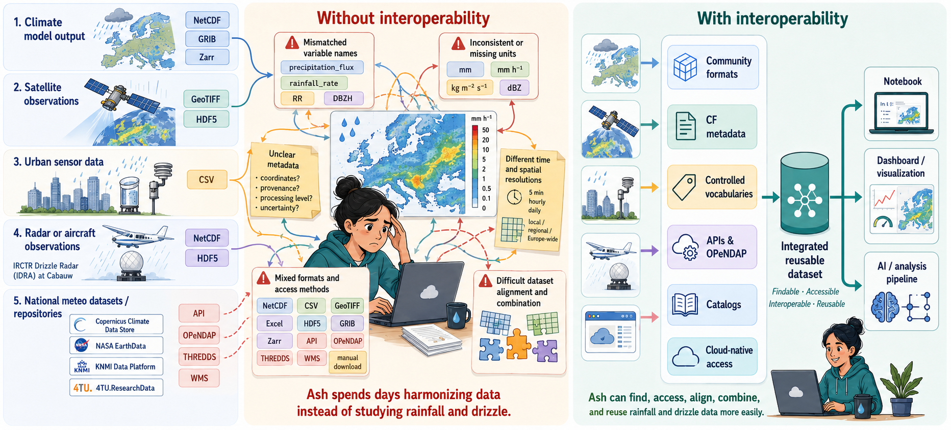
To combine these datasets reliably, Ash needs to answer a sequence of questions:
Can I find the right datasets? Are they described in APIs(Application Programming Interfaces) in a way that supports search by time, location, variable, version, and data type?
Can I read the data structure? Are the files organized using community formats such as NetCDF, Zarr, GeoTIFF, or Parquet, with explicit dimensions, variables, coordinates, and attributes?
Can I understand what the variables mean? Do the datasets use shared metadata conventions, controlled vocabularies, standard names, units, coordinate systems, and provenance information?
Can I access the data programmatically? Can Ash use APIs, OPeNDAP , THREDDS, or other standard access mechanisms instead of downloading everything manually?
Can I work with the data at scale? Can she subset remote files, read only the variables and time periods she needs, or use cloud-native layouts such as Zarr or Kerchunk for repeated analysis?
Can I reproduce and automate the workflow? Are dataset versions, identifiers, metadata, and access routes stable enough for notebooks, dashboards, pipelines, or AI(Artifical Intelligence) workflows?
This lesson follows Ash’s investigation step by step. Learners first diagnose why “open” or “available” data is not automatically interoperable. Then they inspect datasets through the three layers of interoperability:
- Structural interoperability: how data are organized, encoded, and made readable by tools.
- Semantic interoperability: how variables, units, coordinates, and scientific meaning are made clear and machine-actionable.
- Technical interoperability: how data and metadata can be accessed, exchanged, queried, and reused across systems.
References and Glossary
For further reading and definitions of key terms introduced in this workshop, consult the Reference section.
To follow this lesson, learners should already be able to have :
- Working knowledge in Python (write and execute short scripts in Python)
- Awareness of NetCDF format
| Setup Instructions | Download files required for the lesson | |
| Duration: 00h 00m | 1. Introduction |
Why interoperability is important when dealing with research
data? What are the three layers of interoperability? How can you identify if a dataset is interoperable or not? |
| Duration: 01h 00m | 2. Structural interoperability |
What is structural interoperability, and what does it allow software to
do? How do data models, file formats, schemas, conventions, and access methods differ? How can simple tabular formats such as CSV and TSV support reusable, machine-actionable data? Which structural standards are appropriate for common climate and atmospheric data types? What structural contract does the NetCDF data model provide? |
| Duration: 02h 00m | 3. Semantic interoperability |
What is semantic interoperability? What types of meaning must be made explicit to enable semantic interoperability? Why can two structurally similar datasets still be scientifically incompatible? What is the difference between a label, a controlled vocabulary, a code list, and an ontology? Where can researchers discover, evaluate, and share semantic artefacts for the Earth sciences? How do the CF Conventions encode the meaning and context of climate and atmospheric data? Is using the same CF standard_name sufficient to make two variables directly
comparable?What does it mean for a NetCDF file to conform to a particular version of the CF Conventions? What can a CF compliance checker determine, and what are its limitations? |
| Duration: 02h 45m | 4. Technical interoperability: Data access protocols |
What is technical interoperability? What is the difference between storing data remotely and providing remote data access? What is the DAP (Data Access Protocol)? How does OPeNDAP enable remote access without full download? What happens when we open a remote NetCDF file using xarray.open_dataset()?Why are remote data-access protocols important for large-scale scientific workflows? |
| Duration: 03h 30m | 5. Technical interoperability: API |
What is technical interoperability in research data
infrastructures? What is a REST API? How do APIs enable machine-to-machine workflows? How do APIs depend on structural and semantic interoperability? How can we programmatically manage datasets using the 4TU.ResearchData API? |
| Duration: 05h 30m | 6. Cloud-Native Layouts |
What problem are cloud-native data layouts designed to solve? What is object storage, and how does it differ from a traditional filesystem? Why is a conventional NetCDF file not considered a cloud-native layout? How does Zarr organise multidimensional data differently? How do cloud-native layouts affect interoperability? How can Kerchunk bridge existing NetCDF archives and cloud-oriented workflows? |
| Duration: 06h 15m | 7. Interoperable Infrastructure in the AI Era | |
| Duration: 06h 45m | Finish |
The actual schedule may vary slightly depending on the topics and exercises chosen by the instructor.
1. Software Setup
We will use JupyterLab for live coding and exercises.
This course requires:
- A Unix-like terminal
-
uv, a Python package and project manager - Python 3.11 or newer
- Several Python libraries, defined in
pyproject.toml -
jqlibrary - optional for API episode
Install uv (Required)
We use uv instead of manually creating a virtual
environment with venv and installing packages from
requirements.txt.
Install uv using one of the options below.
Alternative installation methods
You can also install uv with package managers such as
Homebrew, Winget, Scoop, or pipx.
See the official installation instructions:
With uv, the main workflow is:
uv sync creates and updates the course
environment.uv run runs commands inside that environment.
You do not need to manually activate the virtual environment during
the course if you use uv run.
Verify uv Installation
Open a terminal and run:
Expected output:
The exact version number may be different.
If your terminal says uv: command not found, close and
reopen the terminal and try again.
If it still does not work, check whether the installation directory
was added to your PATH.
Install or Check Python
This course was tested with Python 3.11.
uv can use an existing Python installation or install
Python for you.
To install Python 3.11 with uv, run:
Then verify that Python is available:
Expected output:
A newer Python 3 version may also work, but Python 3.11 is recommended for the course.
Python 2.7 is not supported.
Please use Python 3.11 or newer.
If you already have Python installed, uv may use your
existing Python version automatically.
2. Project Setup
Create a course working directory somewhere convenient, for example your home directory:
This folder will contain the course environment files, notebooks, scripts, and any downloaded data used during the exercises.
3. Environment Setup
Download the Course Environment File
Make sure you are inside the course folder:
Download the course environment file:
BASH
curl -o pyproject.toml \
https://raw.githubusercontent.com/4TUResearchData-Carpentries/interoperability-climate-sciences/main/learners/files/pyproject.toml
The pyproject.toml file defines the Python dependencies
required for this course.
Verify that the file was downloaded successfully:
Expected output:
Generate the lockfile before the workshop with:
The uv.lock file records the resolved package versions
and improves reproducibility across learners’ machines.
If the download fails, open the download
URL in a web browser and save the file as:
pyproject.toml inside your
Interoperability_climate_sciences folder.
Create and Synchronise the Environment
Run:
This command will:
- create a local
.venvfolder if it does not exist; - install all packages listed in
pyproject.toml; - create or update the
uv.lockfile.
Send this step to participants before the lesson.
The first uv sync can take some time, depending on the
internet connection and operating system.
Recommended pre-workshop instruction:
BASH
cd ~/Interoperability_climate_sciences
curl -o pyproject.toml \
https://raw.githubusercontent.com/4TUResearchData-Carpentries/interoperability-climate-sciences/main/learners/files/pyproject.toml
uv sync
If participants cannot complete this before the lesson, keep a 20-30 minute setup buffer at the beginning of the workshop.
The .venv folder is the virtual environment created by
uv.
Learners do not need to activate it manually if they use commands
starting with uv run.
Verify the Python Environment
Run:
BASH
uv run python -c "import xarray, netCDF4, pydap, zarr, kerchunk, fsspec, h5netcdf, h5py, scipy, pandas, requests, cf_xarray; print('All good')"Expected output:
If this command works, the Python environment for this course is ready.
Register the Environment in Jupyter
Register the course environment as a Jupyter kernel:
BASH
uv run python -m ipykernel install --user --name nes-course-env --display-name "NES Course (Python)"This makes the environment available inside JupyterLab as:
NES Course (Python)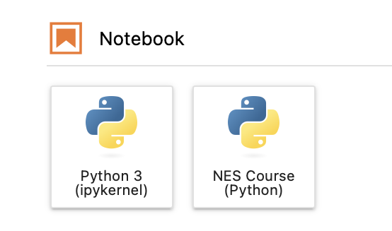
4. Final Setup Check
Before the workshop, make sure the following commands work:
BASH
uv --version
uv run python --version
uv sync
uv run python -c "import xarray, netCDF4, pydap, zarr, kerchunk, fsspec; print('All good')"
uv run jupyter lab
jq --version
If all commands work, you are ready for the course.
5. Troubleshooting
uv: command not found
Close and reopen your terminal.
Then try:
If it still fails, reinstall uv or check whether the
installation folder was added to your PATH.
JupyterLab opens but the course kernel is missing
Run:
BASH
uv run python -m ipykernel install --user --name nes-course-env --display-name "NES Course (Python)"Then restart JupyterLab:
You are not sure which Python is being used
Run:
The executable path should point to the .venv folder
inside your course directory.
Example:
.../Interoperability_climate_sciences/.venv/...Optional Fallback: venv and
requirements.txt
Use this fallback only if uv cannot be installed on your
machine.
The recommended setup for this course is uv.
Use this section only if your institution blocks uv
installation or if you cannot get uv working before the
lesson.
Create a virtual environment:
Activate it.
Install dependencies from a requirements.txt file
provided by the instructors:
Register the environment in Jupyter:
Launch JupyterLab: